There is some indication that Ahmes preferred fractions with even
denominators, because they are easier to double, and the usual
Egyptian method of multiplication required repeated doubling.
Although I had long ago written an article about why the
Rhind mathematical papyrus (RMP) has a table of Egyptian fraction
expansions of !!\frac23, \frac25, \frac27\ldots!! but no similar table
for any other numerator. I had proposed a very reasonable algorithm for how the table of
!!\frac2n!! would give you the ability to compute !!\frac mn!! for any
!!n!!, but for some reason I never connected this in my head with how
the Egyptians actually did multiplication. The Egyptian
multiplication algorithm makes my original surmise very plausible, but
a little bit inside-out.
Also, this blog has somehow never discussed the ancient Egyptian
method of multiplication, which reduces multiplication to addition
without a need for multiplication tables. You don't have to remember
complicated facts like !!7×8=56!!, only simple facts like !!7+7=14!!.
Egyptian multiplication
Let's say we'd like to multiply !!364!! by !!41!!. First let's observe that
it's quites easy to double a number like !!364!!, significantly easier
than to multiply it by anything else. First, !!4+4=8!!, so write
down an !!8!! under the !!4!!:
$$
\begin{array}{}
3 & 6 & 4 \\
& & {\bf 8}
\end{array}
$$
Now !!6+6=12!! so write down a !!2!! under the !!7!! and note a carry in the
next column. Or just remember it until the next step — when doubling,
the carry is never bigger than !!1!!, so we don't have to remember
how much it is, just that there is one:
And yes, !!364+364=728!!, quick and easy. Between each step and the next we only need to
remember one thing: is there a carry? And someone can do the whole thing
with minimal training, knowing only that !!1+1=2, 2+2=4, 3+3=6,\dots, 9+9=18!!.
When the Egyptians wanted to multiply !!364×41!!, they would do a
series of these doublings, and label each one (perhaps just mentally) with the corresponding
power of 2:
Then they'd find the numbers in the left-hand column that added to 41,
and mark them. This is easy to do, using the greedy method:
!!32 < 41!!, so mark the !!32!!, then subtract !!41-32=9!! and
proceed up to the next line. !!16\not\lt 9!!, so don't mark the
!!16!!, but do mark the !!8!!, and so on:
And that's the answer, !!364 \times 41 = 14924!!.
Isn't that cute?
The algorithm is really quite practical. It is often known as the
Russian Peasant algorithm, apparently because it was also used by
actual Russian peasants.
Once again, with fractions
Now fractions. Say we want to multiply !!4+\frac{1}{35}!! by !!29!!.
The !!4!! we already know how to do and it is easy enough, we just do
it like above, doubling !!4!! repeatedly and adding the correct
doubles. Or if we're even a little clever we realize we can do
it by doubling !!29!! twice, which is quicker.
But Egyptian notation for fractions was terrible. They had a notation
for !!\frac1{35}!!, and a special notation for !!\frac 23!!, but no
general quotient operation like the fraction bar. Instead they wrote
fractions as sums of “unit fractions” with numerator !!1!!, and they
had tables like the one in the Rhind Mathematical Papyrus, for
converting non-unit fractions to sums of unit fractions, for example
$$\frac2{35} = \frac1{30} + \frac1{42}.$$
!!\def\uf#1.{\frac1{#1}}\def\u#1.{\uf#1.}!!
So now we want to multiply !!19\times \frac1{35}!!. Per the
algorithm we need to double !!\frac1{35}!! four times until we get
!!\uf35. \times 16!!. For
the first doubling we go to the table for !!\frac2{35}!!:
For the next doubling, we don't have to go to the table, because the
double of !!\uf30.!! is just !!\uf15.!! and the double of !!\uf42.!!
is !!\uf21.!!. That's why the table prefers expansions with even denominators.
There are duplicates of !!\color{darkgreen}{\u15.}!! and !!\color{purple}{\u21.}!! and that's not
allowed, so we use the !!\frac2n!! table to replace the
!!\color{darkgreen}{\u15.+\u15.}!! with !!\u10.+\u30.!! and the
!!\color{purple}{\u21.+\u21.}!! with !!\u14.+\u42.!!:
and we are finally done, having discovered that !!\frac{29}{35} =
\u3. + \u4. + \u10. + \u21. + \u28. + \u30.!!. Wow.
A slightly cleverer method would be to observe that !!29\times\u35. =
\u35. +
28\times\u35. !!, and that !!28\times\u35. !! is simply !! 4\times \u5.!!. I
imagine that a competent Egyptian scribe would have noticed this.
Did they really do this?
Wikipedia hints that perhaps the Egyptian didn't actually do go
through all of this trouble, that perhaps they computed
!!\frac{29}{35}!! first the way we did, as a vulgar fraction, and then
only converted to the awful sum-of-unit-fractions notation when they
needed to record the final answer.
This would have been analogous to how for hundreds of years Europeans
would convert awful Roman numerals into an arrangement of counting
board tokens (an abacus, essentially), do the calculation on the
counting board, and then convert back to awful Roman numerals to
record the answer.
While prearing this article I wondered: how can we even be sure that
the algorithm will terminate? It's not clear to me. There was that
point where we got rid of a !!\frac2{15}!! and then it came back and
we had to get rid of it again.
I had Claude implement the algorithm, using the actual RMP !!\frac2n!!
table, and run it for every product up to !!100\times \u101.!! to see if it
would get stuck in any loops. It didn't.
It's possible that it would have looped if the !!\frac2n!! table I
used had been a little different, and it would be very interesting to
learn if the table itself had been somehow constructed so as to
prevent the algorithm from looping. But I think it's more likely that
it terminates for any reasonable !!\frac2n!! table, because the
algorithm has some invariant that always decreases — one which I'm not
yet clever enough to see.
I mentioned in the previous article:
The Egyptians, like everyone, often had to multiply by 10.
Most of the really big denominators in the !!\frac2n!! table are
multiples of !!10!!. For example it has !!\frac2{47} = \u30. + \u141. +
\u470.!! and if you're multiplying by !!2!! or even by !!10!!, only the
middle part of this is any trouble. I wouldn't want to multiply
!!10\times\u141.!! by the algorithm above, though — the !!\frac2n!! table doesn't even go that
high. But maybe they would have done something like:
!!10\times \u141. = 10\times(\u3. \times \u47)
This whole thing raises a big question for me. To have useful
numbers, you need three things:
Addition
Multiplication
Comparison
People often forget #3, but it is crucial, because in the real world
you are using the numbers to answer questions like “do we have enough
bread to feed 119 laborers for 21 days?” or “will the bridge
hold if I drive two loaded ox-carts across it” or similar questions
that involve comparisons.
Say we're trying to figure out how to divide nine heaps of grain among
!!99!! workers. Supposing that you had somehow failed to notice that
the answer was !!\u11.!!, you might use
the multiplication algorithm above, and after some grinding it would
tell you that:
$$\frac9{99} = \u22. + \u33. + \u99. + \u198.$$
This is a useless answer because the !!\u198.!! means that you should
start by taking half of one heap and dividing it into !!99!! equal
shares of !!\u198.!! heap for each worker. This is impractical to say
the least. So there must be some way to recognize that
!!\u22. + \u33. + \u99. + \u198.!! is ⸢actually⸣ !!\u11.!!.
The ancient Egyptians had a terrible notation for fractions. They had
notations for !!\u n!! for each !!n!!, for !!\frac23!!, but everything
else was written as a sum of these, with repeats forbidden, so that
for example !!\frac25!! had to be written as !!\u3 +
\u{15}!!. (Wikipedia)
Getting the table of good-quality representations of !!\frac2n!! is
not trivial, and requires searching, number theory, and some trial
and error. It's not at all clear that !!\frac2{105}=\u{90} + \u{126}!!.
I think I see now where this comes from. !!105 = 3·7·5!!, so two of
the summands must have denominators divisible by !!5!! and by !!7!!
respectively. The first thing you should do is consider $$\u5 + \u7
= \frac{12}{35} = \frac{36}{105}.$$
But you don't want !!\frac{36}{105}!!, you want !!\frac{2}{105}!!, so
you multiply by !!\u{18}!!:
Why pick !!\u5!! and !!\u7!! rather than, say, !!\u3!! and
!!\u5!!? I suspect the answer is probably: Ahmes (or someone
earlier) tried it both ways and picked the result they liked best.
Remember Ahmes is compiling a reference table here, so he does these
calculations once, writes down the best result, and throws the others
away.
If you do the same trick with !!3!! and !!5!! instead you get
!!\u3+\u5 = \frac8{15} = \frac{56}{105}!!. Then you multiply
everything by !!\u{28}!! producing $$\u{84} + \u{140} =
\frac2{105}$$ which seems a little worse than the other one. Using
the !!3!! and the !!5!! produces $$\u{75} + \u{175} =
\frac2{105}$$ which seems much worse.
Of course this only works when the denominator is composite.
Here's another approach, which doesn't work too well in this case but
might be useful for other examples. Consider that !!\frac23 =
\u2 + \u6!!. We want !!\frac2{105} =
\u{35}\cdot\frac23!!. So
The denominators here are a lot bigger than the first expansion, but
they do at least have the advantage of being multiples of !!10!!.
The Egyptians like this because they, like us, often need to multiply
numbers by !!10!!, and whereas a fraction like !!\u{126}!! is hard for
them to multiply by !!10!!, it's trivial to multiply !!\u{210}!! by !!10!!.
A couple of years back I was discussing the Rhind Mathematical Papyrus
(RMP). It includes a table expressing !!\frac 2n!! as a sum
$$\frac1{a_1}+\frac1{a_2}+\dots+\frac1{a_k} $$ fractions with
numerator 1 (“unit fractions”). I said:
Getting the table of good-quality representations of !!\frac 2n!! is not
trivial, and requires searching, number theory, and some trial and
error. It's not at all clear that !!\frac2{105}=\frac1{90} +
\frac1{126}!!.
Today I wondered: did Ahmes (the author) have the best possible
expansions for all the !!\frac2n!! values, or were there some
improvements the Egyptians had missed?
but !!\frac1{380} + \frac1{570} = \frac1{228}!! so it could have been
written as $$\frac2{95} = \frac1{60}+\frac1{228}.$$
But wait, maybe that wasn't an error. The Egyptians, like everyone,
often had to multiply by 10. (In fact, the RMP itself, right after
its !!\frac 2n!! table, has a shorter table of expansions of !!\frac
n{10}!!.) And !!\frac1{60} + \frac1{380} + \frac1{570}!! is trivially
multiplied by 10, whereas !!\frac1{228}!! isn't. There is some
indication that Ahmes preferred fractions with even denominators,
because they are easier to double, and the usual Egyptian method of
multiplication required repeated doubling. But the Egyptians also
sometimes decupled while multiplying, and the !!\frac1{60} +
\frac1{380} + \frac1{570}!! expansion would have made both of those
easy.
The methods by which Ahmes chose the expansions of !!\frac 2n!!, and
the criteria by which he preferred one to another, are still unknown;
he doesn't explain them. So it's tough to say that any item was or
wasn't “best” from Ahmes' point of view.
Mathematical folklore contains a story about how Acta Quandalia
published a paper proving that all partially uniform k-quandles had
the Cosell property, and then a few months later published another
paper proving that no partially uniform k-quandles had the Cosell
property. And in fact, goes the story, both theorems were quite
true, which put a sudden end to the investigation of partially
uniform k-quandles.
My main dissertation result was a conditional result. And about
four years after I graduated, a Hungarian graduate student proved
that my condition, like my additional hypothesis, held in only
trivial cases.
(At 04:15)
In the earlier article, I had said:
Suppose you had been granted a doctorate on the strength of your
thesis on the properties of objects from some class which was
subsequently shown to be empty. Wouldn't you feel at least a bit
like a fraud?
In the podcast, Alm introduces this as evidence that he “wasn't very
good at algebra”. Fortunately, he added, it was after he had
graduated.
The episode title is “In Which Every Thing Happens or it Doesn't”. I
started listening to it because I expected it to be about the
ergodic theorem, and I'd like to understand the
ergodic theorem. But it turned out to be
about the Rado graph. This is
fine with me, since I love the Rado graph. (Who doesn't?)
Suppose a centrifuge has !!n!! slots, arranged in a circle around the
center, and we have !!k!! test tubes we wish to place into the slots.
If the tubes are not arranged symmetrically around the center, the
centrifuge will explode.
(By "arranged symmetrically around the center, I mean that if the
center is at !!(0,0)!!, then the sum of the positions of the tubes
must also be at !!(0,0)!!.)
Let's consider the example of !!n=12!!. Clearly we can arrange !!2!!,
!!3!!, !!4!!, or !!6!! tubes symmetrically:
Equally clearly
we can't arrange only !!1!!. Also it's easy to see we can do !!k!! tubes if
and only if we can also do !!n-k!! tubes, which rules out !!n=12,
k=11!!.
From now on I will write !!\nk nk!! to mean the problem of balancing
!!k!! tubes in a centrifuge with !!n!! slots. So !!\dd 2, \dd 3, \dd
4, !! and !!\dd 6!! are possible, and !!\dd 1!! and !!\dd{11}!! are
not. And !!\nk nk!! is solvable if and only if !!\nk n{n-k}!! is.
It's perhaps a little surprising that !!\dd7!! is possible.
If you just ask this to someone out of nowhere they might
have a happy inspiration: “Oh, I'll just combine the solutions for
!!\dd3!! and !!\dd4!!, easy.” But that doesn't work because two groups
of the form !!3i+j!! and !!4i+j!! always overlap.
For example, if your group of !!4!! is the
slots !!0, 3, 6, 9!! then you can't also have your group of !!3!! be
!!1, 5, 9!!, because slot !!9!! already has a tube in it.
The
other balanced groups of !!3!! are blocked in the same way. You
cannot solve the puzzle with !!7=3+4!!; you have to do !!7=3+2+2!! as
below left.
The best way to approach this is to do !!\dd5!!, as below right.
This is easy,
since the triangle only blocks three of the six symmetric pairs.
Then you replace the holes with tubes and the tubes with holes to
turn !!\dd5!! into !!\dd{12-5}=\dd7!!.
Given !!n!! and !!k!!, how can we decide whether the centrifuge can be
safely packed?
Clearly you can solve !!\nk nk!! when !!n!! is a multiple of !!k>1!!, but the example
of !!\dd5!! (or !!\dd7!!) shows this isn't a necessary condition.
A generalization of this is that !!\nk nk!! is always solvable
if !!\gcd(n,k) > 1!! since you can easily
balance !!g = \gcd(n, k)!! tubes at positions !!0, \frac ng, \frac{2n}g, \dots,
\frac {(g-1)n}g!!, then do another !!g!! tubes one position over, and
so on. For example, to do !!\dd8!! you just put first four tubes
in slots !!0, 3, 6, 9!! and the next four one position over, in slots
!!1, 4, 7, 10!!.
An interesting counterexample is that the strategy for !!\dd7!!,
where we did !!7=3+2+2!!, cannot be extended to !!\nk{14}9!!. One
would want to do !!k=7+2!!, but there is no way to arrange the tubes
so that the group of !!2!! doesn't conflict with the group of !!7!!,
which blocks one slot from every pair.
But we can see that this must be true without even considering the
geometry. !!\nk{14}9!! is the reverse of !!\nk{14}{14-9} = \nk{14}5!!, which
impossible: the only nontrivial divisors of !!n=14!! are !!2!! and
!!7!!, so !!k!! must be a sum of !!2!!s and !!7!!s, and !!5!! is not.
You can't fit !!k=3+5=8!! tubes when !!n=15!!, but again the reason is
a bit tricky. When I looked at !!8!! directly, I did a case analysis
to make sure that the !!3!!-group and the !!5!!-group would always
conflict. But again there was an easier was to see this: !!8=15-7!! and
!!7!! clearly won't work, as !!7!! is not a sum of !!3!!s and !!5!!s.
I wonder if there's an example where both !!k!! and !!n-k!! are not obvious?
For !!n=20!!, every !!k!! works except !!k=3,17!! and the always-impossible !!k=1,19!!.
What's the answer in general? I don't know.
Addenda
20250502
Now I am amusing myself thinking about the perversity of a centrifuge
with a prime number of slots, say !!13!!. If you use it at all, you must
fill every slot. I hope you like explosions!
While I did not explode any centrifuges in university chemistry, I did
once explode an expensive Liebig condenser.
Omar Antolín points out an important consideration I missed:
it may be necessary
to subtract polygons. Consider !!\nk{30}6!!. This is obviously
possible since !!6\mid 30!!. But there is a more interesting
solution. We can add the pentagon !!{0, 6, 12, 18, 24}!! to the
digons !!{5, 20}!! and !!{10, 25}!! to obtain the solution
$${0,5,6,10,12,18, 20, 24, 25}.$$
Then from this we can subtract the triangle !!{0, 10,
20}!! to obtain $${5, 6, 12, 18, 24, 25},$$ a solution to
!!\nk{30}6!! which is not a sum of regular polygons:
Thanks to Dave Long for pointing out a small but significant error,
which I have corrected.
Given the coordinates of the three vertices of a triangle, can we find
the area? Yes. If by no other method, we can use the Pythagorean
theorem to find the lengths of the edges, and then
Heron's formula to compute the area from
that.
Now, given the coordinates of the four vertices of a quadrilateral,
can we find the area? And the answer is, no, there is no method to do
that, because there is not enough information:
These three quadrilaterals have the same vertices, but different
areas. Just knowing the vertices is not enough; you also need their order.
I suppose one could abstract this: Let !!f!! be the function that maps
the set of vertices to the area of the quadrilateral. Can we
calculate values of !!f!!? No, because there is no such !!f!!, it is
not well-defined.
Put that way it seems less interesting. It's just another example of
the principle that, just because you put together a plausible sounding
description of some object, you cannot infer that such an object must
exist. One of the all-time pop hits here is:
Let !!ε!! be the smallest [real / rational] number strictly greater than !!0!!…
which appears on Math SE quite frequently. Another one I remember is
someone who asked about
the volume of a polyhedron with exactly five faces, all triangles. This
is a fallacy at the ontological level, not the mathematical
level, so when it comes up I try to demonstrate it with a
nonmathematical counterexample, usually something like “the largest
purple hat in my closet” or perhaps “the current Crown Prince of the
Ottoman Empire”. The latter is less good because it relies on the
other person to know obscure stuff about the Ottoman Empire, whatever
that is.
This is also unfortunately also the error in Anselm's so-called
“ontological proof of God”. A philosophically-minded friend of mine
once remarked that being known for the discovery of the ontological
proof of God is like being known for the discovery that you can wipe
your ass with your hand.
Anyway, I'm digressing. The interesting part of the quadrilateral
thing, to me, is not so much that !!f!! doesn't exist, but the specific
reasoning that demonstrates that it can't exist. I think there are
more examples of this proof strategy, where we prove nonexistence
by showing there is not enough information for the thing to exist, but
I haven't thought about it enough to come up with one.
There is a proof, the so-called
“information-theoretic proof”,
that a comparison sorting algorithm takes at least !!O(n\log n)!! time, based
on comparing the amount of information gathered from the comparisons
(one bit each) with that required to distinguish all !!n! !! possible
permutations (!!\log_2 n! \ge n\log_2 n!! bits total). I'm not sure
that's what I'm looking for here. But I'm also not sure it isn't, or
why I feel it might be different.
Addenda
20250430
Carl Muckenhoupt suggests that logical independence proofs are of the
same sort. He says, for example:
Is there a way to prove the parallel postulate from Euclid's other
axioms? No, there is not enough information. Here are two geometric
models that produce different results.
This is just the sort of thing I was looking for.
20250503
Rik Signes has allowed me to reveal that he was the source of the
memorable disparagement of Anselm's dumbass argument.
A modern presentation of the Peano axioms looks like
this:
!!0!! is a natural number
If !!n!! is a natural number, then so is the result of appending an
!!S!! to the beginning of !!n!!
Nothing else is a natural number
This baldly states that zero is a natural number.
I think this is a 20th-century development. In 1889, the natural
numbers started at !!1!!, not at !!0!!. Peano's
Arithmetices principia, nova methodo exposita
(1889) is the source of the Peano axioms and in it Peano starts the
natural numbers at !!1!!, not at !!0!!:
There's axiom 1: !!1\in\Bbb N!!. No zero. I think starting at !! 0!!
may be a Bourbakism.
In a modern presentation we define addition like this:
$$
\begin{array}{rrl}
(i) & a + 0 = & a \\
(ii) & a + Sb = & S(a+b)
\end{array}
$$
Peano doesn't have zero, so he doesn't need item !!(i)!!. His definition
just has !!(ii)!!.
But wait, doesn't his inductive definition need to have a base case? Maybe something like this?
\begin{array}{rrl}
(i') & a + 1 = & Sa \\
\end{array}
Nope, Peano has nothing like that. But surely the definition must
have a base case? How can Peano get around that?
Well, by modern standards, he cheats!
Peano doesn't have a special notation like !!S!! for successor. Where
a modern presentation might write !!Sa!! for the successor of the
number !!a!!, Peano writes “!!a + 1!!”.
So his version of !!(ii)!! looks like this:
$$
a + (b + 1) = (a + b) + 1
$$
which is pretty much a symbol-for-symbol translation of !!(ii)!!. But
if we try to translate !!(i')!! similarly, it looks like this:
$$
a + 1 = a + 1
$$
That's why Peano didn't include it: to him, it was tautological.
But to modern eyes that last formula is deceptive because it
equivocates between the "!!+ 1!!" notation that is being used to
represent the successor operation (on the right) and the addition
operation that Peano is trying to define (on the left). In a modern
presentation, we are careful to distinguish between our formal symbol
for a successor, and our definition of the addition operation.
Peano, working pre-Frege and pre-Hilbert, doesn't have the same
concept of what this means. To Peano, constructing the successor of a
number, and adding a number to the constant !!1!!, are the same
operation: the successor operation is just adding !!1!!.
But to us, !!Sa!! and !!a+S0!! are different operations that happen to
yield the same value. To us, the successor operation is a purely
abstract or formal symbol manipulation (“stick an !!S!! on the
front”). The fact that it also has an arithmetic interpretation,
related to addition, appears only once we contemplate the theorem
$$\forall a. a + S0 = Sa.$$ There is nothing like this in Peano.
It's things like this that make it tricky to read older mathematics
books. There are deep philosophical differences about what is being
done and why, and they are not usually explicit.
Another example: in the 19th century, the abstract presentation of
group theory had not yet been invented. The phrase “group” was
understood to be short for “group of permutations”, and the important
property was closure, specifically closure under composition of
permutations. In a 20th century abstract presentation, the closure
property is usually passed over without comment. In a modern view, the
notation !!G_1\cup G_2!! is not even meaningful, because groups are
not sets and you cannot just mix together two sets of group elements
without also specifying how to extend the binary operation, perhaps
via a free product or something. In the 19th century, !!G_1\cup G_2!!
is perfectly ordinary, because !!G_1!! and !!G_2!! are just sets of
permutations. One can then ask whether that set is a group — that is,
whether it is closed under composition of permutations — and if not,
what is the smallest group that contains it.
It's something like a foreign language of a foreign
culture. You can try to translate the words, but the underlying ideas
may not be the same.
Addendum 20250326
Simon Tatham reminds me that Peano's equivocation has come up here
before.
I previously discussed
a Math SE post
in which OP was confused
because Bertrand Russell's presentation of the Peano axioms similarly
used the notation “!!+ 1!!” for the successor operation, and did not
understand why it was not tautological.
Here's a Math SE pathology that bugs me. OP will ask "I'm trying
to prove that groups !!A!! and !!B!! are isomorphic, I constructed this
bijection but I see that it's not a homomorphism. Is it sufficient,
or do I need to find a bijective homomorphism?"
And respondent !!R!! will reply in the comments "How can a function which is
not an homomorphism prove that the groups are isomorphic?"
Which is literally the exact question that OP was asking! "Do I need
to find … a homomorphism?"
My preferred reply would be something like "Your function is not
enough. You are correct that it needs to be a homomorphism."
Because what problem did OP really have? Clearly, their problem is
that they are not sure what it means for two groups to be isomorphic.
For the respondent to ask "How can a function which is not an
homomorphism prove the the groups are isomorphic" is unhelpful because
they know that OP doesn't know the answer to that question.
OP knows too, that's exactly what their question was! They're trying
to find out the answer to that exact question! OP correctly
identified the gap in their own understanding. Then they formulated a
clear, direct question that would address the gap.
THEY ARE ASKING THE EXACT RIGHT QUESTION AND !!R!! DID NOT ANSWER IT
My advice to people answering questions on MSE:
Just answer the question
It's all very well for !!R!! to imagine that they are going to be
brilliant like Socrates, conducting a dialogue for the ages that draws from OP the
realization that the knowledge they sought was within them all along.
Except:
!!R!! is not Socrates
Nobody has time for this nonsense
The knowledge was not within them all along
MSE is a site where people go to get answers to their questions. That
is its sole and stated purpose. If !!R!! is not going to answer
questions, what are they even doing there? In my opinion, just
wasting everyone's time.
Important pedagogical note
It's sufficient to say "Your function is not enough", which answers
the question.
But it is much better to say "Your function is not enough. You are
correct that it needs to be a homomorphism". That acknowledges the
student's contribution. It tells them that their analysis of the
difficulty was correct!
They may not know what it means for two groups to be isomorphic, but
they do know one something almost as good: that they are unsure what
it means for two groups to be isomorphic. This is valuable knowledge.
This wise student recognises that they don't know. Socrates said that
he was the wisest of all men, because he at least “knew that he didn't
know”. If you want to take a lesson from Socrates, take that one, not
his stupid theory that all knowledge is already within us.
OP did what students are supposed to do: they reflected on their
knowledge, they realized it was inadequate, and they set about
rectifying it. This deserves positive reinforcement.
Addenda
This is a real example. I have not altered it, because I am afraid
that if I did you would think I was exaggerating.
I have been banging this drum for decades, but I will cut the
scroll here. Expect a followup article.
This post is about the bottom center panel, “Game Theory final exam”.
I don't know much about game theory and I haven't seen any other
discussion of this question. But I have a strategy I think is
plausible and I'm somewhat pleased with.
(I assume that answers to the exam question must be real numbers — not
!!\infty!! — and
that “average” here is short for 'arithmetic mean'.)
First, I believe the other players and I must find a way to agree on
what the average will be, or else we are all doomed. We can't
communicate, so we should choose a Schelling point and hope that
everyone else chooses the same one. Fortunately, there is only one
distinguished choice: zero. So I will try to make the average zero
and I will hope that others are trying to do the same.
If we succeed in doing this, any winning entry will therefore be
!!10!!. Not all !!n!! players can win because the average must be
!!0!!. But !!n-1!! can win, if the one other player writes
!!-10(n-1)!!. So my job is to decide whether I will be the loser. I
should select a random integer between !!0!! and !!n-1!!. If it is
zero, I have drawn a short straw, and will write
!!-10(n-1)!!. otherwise I write !!10!!.
(The straw-drawing analogy is perhaps misleading. Normally, exactly
one straw is short. Here, any or all of the straws might be short.)
If everyone follows this strategy, then I will win if exactly one
person draws a short straw and if that one person isn't me. The
former has a probability that rapidly approaches !!\frac1e\approx
36.8\%!! as !!n!! increases, and the latter is !!\frac{n-1}n!!. In an !!n!!-person class,
the probability of my winning is $$\left(\frac{n-1}n\right)^n$$ which
is already better than !!\frac13!! when !!n= 6!!, and it increases slowly
toward !!36.8\%!! after that.
Some miscellaneous thoughts:
The whole thing depends on my idea that everyone will agree on
!!0!! as a Schelling point. Is that even how Schelling points
work? Maybe I don't understand Schelling points.
I like that the probability !!\frac1e!! appears. It's surprising
how often this comes up, often when multiple
agents try to coordinate without communicating. For example, in
ALOHAnet a number of ground
stations independently try to send packets to a single satellite
transceiver, but if more than one tries to send a packet at a
particular time, the packets are garbled and must be retransmitted.
At most !!\frac1e!! of the available bandwidth can be used, the
rest being lost to packet collisions.
The first strategy I thought of was plausible but worse: flip a
coin, and write down !!10!! if it is heads and !!-10!! if it is
tails. With this strategy I win if exactly !!\frac n2!! of the
class flips heads and if I do too. The probability of this
happening is only $$\frac{n\choose n/2}{2^n}\cdot \frac12 \approx
\frac1{\sqrt{2\pi n}}.$$ Unlike the other strategy, this decreases to
zero as !!n!! increases, and in no case is it better than the
first strategy. It also fails badly if the class contains an odd
number of people.
Just because this was the best strategy I could think of in no way
means that it is the best there is. There might have been
something much smarter that I did not think of, and if there is
then my strategy will sabotage everyone else.
Going in the other direction, even if !!n-1!! of the smartest
people all agree on the smartest possible strategy, if the !!n!!th
person is Leeroy Jenkins, he is going to ruin it for everyone.
If I were grading this exam, I might give full marks to anyone who
wrote down either !!10!! or !!-10(n-1)!!, even if the average came
out to something else.
For a similar and also interesting but less slippery question, see
Wikipedia's article on
Guess ⅔ of the average. Much of
the discussion there is directly relevant. For example, “For Nash
equilibrium to be played, players would need to assume both that
everyone else is rational and that there is common knowledge of
rationality. However, this is a strong assumption.” LEEROY
JENKINS!!
People sometimes suggest that the real Schelling point is for
everyone to write !!\infty!!. (Or perhaps !!-\infty!!.)
Feh.
If the class knows ahead of time what the question will be, the
strategy becomes a great deal more complicated! Say there are six
students. At most five of them can win. So they get together and
draw straws to see who will make a sacrifice for the common good.
Vidkun gets the (unique) short straw, and agrees to write !!-50!!. The
others accordingly write !!10!!, but they discover that instead of
!!-50!!, Vidkun has written !!22!! and is the only person to have guessed
correctly.
I would be interested to learn if there is a playable Nash
equilibrium under these circumstances. It might be that the
optimal strategy is for everyone to play as if they didn't know
what the question was beforehand!
Suppose the players agree to follow the strategy I outlined, each
rolling a die and writing !!-50!! with probability !!\frac16!!, and
!!10!! otherwise. And suppose that although the others do this,
Vidkun skips the die roll and unconditionally writes !!10!!. As
before, !!n-1!! players (including Vidkun) win if exactly one of
them rolls zero. Vidkun's chance of winning increases. Intuitively,
the other players' chances of winning ought to decrease. But by
how much? I think I keep messing up the calculation because I keep
getting zero. If this were actually correct, it would be a
fascinating paradox!
Like almost everyone except Alexander Grothendieck, I understand
things better with examples. For instance, how do you explain that
$$(f\circ g)^{-1} = g^{-1} \circ f^{-1}?$$
Oh, that's easy. Let !!f!! be putting on your shoes
and !!f^{-1}!! be taking off your shoes.
And let !!g!! be
putting on your socks and !!g^{-1}!! be taking off your socks.
Now !!f\circ g!! is putting on your socks and then your shoes. And
!!g^{-1} \circ f^{-1}!! is taking off your shoes and then your
socks. You can't !!f^{-1} \circ g^{-1}!!, that says to take your
socks off before your shoes.
(I see a topologist jumping up and down in the back row, desperate to
point out that the socks were never inside the shoes to begin with.
Sit down please!)
Sometimes operations commute, but not in general. If you're teaching
group theory to high school students and they find nonabelian
operations strange, the shoes-and-socks example is an unrebuttable
demonstration that not everything is abelian.
(Subtraction is not a good example here, because subtracting !!a!!
and then !!b!! is the same as subtracting !!b!! and then !!a!!. When
we say that subtraction isn't commutative, we're talking about
something else.)
Anyway this weekend I was thinking about very very elementary
category theory (the only kind I know) and about left and right
inverses. An arrow !!f : A\to B!! has a left inverse !!g!! if
$$g\circ f = 1_A.$$
Example of this are easy. If !!f!! is putting on your shoes, then
!!g!! is taking them off again. !!A!! is the state of shoelessness
and !!B!! is the state of being shod. This !!f!! has a left inverse
and no right inverse. You can't take the shoes off before you put
them on.
But I wanted an example of an !!f!! with right inverse and no left inverse:
$$f\circ h = 1_B$$
and I was pretty pleased when I came up with one involving pouring the
cream pitcher into your coffee, which has no left inverse that gets
you back to black coffee. But you can ⸢unpour⸣ the cream if you do it
before mixing it with the coffee: if you first put the cream back
into the carton in the refrigerator, then the pouring does get you to
black coffee.
But now I feel silly. There is a trivial theorem that if !!g!! is a
left inverse of !!f!!, then !!f!! is a right inverse of !!g!!. So
the shoe example will do for both. If !!f!! is putting on your shoes,
then !!g!! is taking them off again. And just as !!f!! has a left
inverse and no right inverse, because you can't take your shoes off
before putting them on, !!g!! has a right inverse (!!f!!) and no left inverse,
because you can't take your shoes off before putting them on.
This reminds me a little of the time I tried to construct an example
to show that “is a blood relation of" is not a transitive relation. I
had this very strange and elaborate example involving two sets of
sisters-in-law. But the right example is that almost everyone is the
blood relative of both of their parents, who nevertheless are not
(usually) blood relations.
Looking at license plates the other day I noticed that if you have a
four-digit number !!N!! with digits !!abbc!!, and !!a+c=b!!, then
!!N!! will always be a multiple of !!37!!. For example, !!4773 =
37\cdot 129!! and !!1776 = 37\cdot 48!!.
Mathematically this is uninteresting. The proof is completely
trivial. (Such a number is simply !!1110a +111c!!, and
!!111=3\cdot 37!!.)
But I thought that if someone had pointed this out to me when I was
eight or nine, I would have been very pleased. Perhaps if you have a
mathematical eight- or nine-year-old in your life, they will be
pleased if you share this with them.
The principle of explosion is that in an inconsistent system
everything is provable: if you prove both !!P!! and not-!!P!! for
any !!P!!,
you can then conclude !!Q!! for any !!Q!!:
$$(P \land \lnot P) \to Q.$$
This is, to put it briefly, not intuitive. But it is awfully hard
to get rid of because it appears to follow immediately from two
principles that are intuitive:
If we can prove that !!A!! is true, then we can prove that at least
one of !!A!! or !!B!! is true. (In symbols, !!A\to(A\lor B)!!.)
If we can prove that at least one of !!A!! or !!B!! is true, and we
can prove that !!A!! is false, then we may conclude that that !!B!! is
true. (Symbolically, !!(A\lor B) \to (\lnot A\to B)!!.).
Then suppose that we have proved that !!P!! is both true and false.
Since we have proved !!P!! true, we have proved that at least one of
!!P!! or !!Q!! is true. But because we have also proved that !!P!! is
false, we may conclude that !!Q!! is true. Q.E.D.
This proof is as simple as can be. If you want to get rid of this, you
have a hard road ahead of you. You have to follow Graham Priest into
the wilderness of paraconsistent logic.
Raymond Smullyan observes that although logic is supposed to model
ordinary reasoning, it really falls down here. Nobody, on discovering
the fact that they hold contradictory beliefs, or even a false one,
concludes that therefore they must believe everything. In fact,
says Smullyan, almost everyone does hold contradictory beliefs. His
argument goes like this:
Consider all the things I believe individually, !!B_1, B_2,
\ldots!!. I believe each of these, considered separately, is true.
However, I also believe that I'm not infallible, and that at
least one of !!B_1, B_2, \ldots!! is false, although I don't know
which ones.
Therefore I believe both !!\bigwedge B_i!! (because I believe each
of the !!B_i!! separately) and !!\lnot\bigwedge B_i!! (because I
believe that not all the !!B_i!! are true).
And therefore, by the principle of explosion, I ought to believe that
I believe absolutely everything.
Well anyway, none of that was exactly what I planned to write about.
I was pleased because I noticed a very simple, specific example of
something I believed that was clearly inconsistent. Today I learned
that K2, the second-highest mountain in the world, is in
Asia, near the border of Pakistan and westernmost China. I was
surprised by this, because I had thought that K2 was in Kenya
somewhere.
But I also knew that the highest mountain in Africa was
Kilimanjaro. So my simultaneous beliefs were flatly contradictory:
K2 is the second-highest mountain in the world.
Kilimanjaro is not the highest mountain in the world, but it is the
highest mountain in Africa
K2 is in Africa
Well, I guess until this morning I must have believed everything!
How many different ways are there to color the vertices of the
icosahedron with 3 colors such that no two adjacent vertices have
the same color?
I would love to know what was going on here. Is this homework? Just
someone idly wondering?
Because the interesting thing about this question is (assuming that
the person knows what an icosahedron is, etc.) it should be solvable
in sixty seconds by anyone who makes the least effort. If you don't
already see it, you should try. Try what? Just take an icosahedron,
color the vertices a little, see what happens. Here, I'll help you
out, here's a view of part of the end of an icosahedron, although I
left out most of it. Try to color it with 3 colors so that no two
adjacent vertices have the same color, surely that will be no harder
than coloring the whole icosahedron.
The explanation below is a little belabored, it's what OP
would have discovered in seconds if they had actually tried the
exercise.
Let's color the middle vertex, say blue.
The five vertices around the edge can't be blue, they must be the
other two colors, say red and green, and the two colors must alternate:
Ooops, there's no color left for the fifth vertex.
The phrasing of the question, “how many” makes the problem sound
harder than it is: the answer is zero because we can't even color
half the icosahedron.
If OP had even tried, even a little bit, they could have discovered
this. They didn't need to have had the bright idea of looking at a a
partial icosahedron. They could have grabbed one of the pictures from
Wikipedia and started coloring the vertices. They would have gotten
stuck the same way. They didn't have to try starting in the middle of
my diagram, starting at the edge works too: if the top vertex is blue,
the three below it must be green-red-green, and then the bottom two
are forced to be blue, which isn't allowed. If you just try it, you
win immediately. The only way to lose is not to play.
Before the post was deleted I suggested in a comment “Give it a try,
see what happens”. I genuinely hoped this might be helpful. I'll
probably never know if it was.
Like I said, I would love to know what was going on here. I think
maybe this person could have used a dose of Lower Mathematics.
Just now I wondered for the first time: what would it look like if I
were to try to list the principles of Lower Mathematics? “Try it and
see” is definitely in the list.
Then I thought: How To Solve It has that sort of list and something like “try it
and see” is
probably on it. So I took it off the shelf and found: “Draw a
figure”, “If you cannot solve the proposed problem”, “Is it possible
to satisfy the condition?”. I didn't find anything called “fuck
around with it and see what you learn” but it is probably in there
under a different name, I haven't read the book in a long time. To
this important principle I would like to add “fuck around with it and
maybe you will stumble across the answer by accident” as happened
here.
Mathematics education is too much method, not enough heuristic.
Sometime around 1986 or so I considered the question of the dimensions
that a closed cuboidal box must have to enclose a given volume
but use as little material as possible. (That is, if its surface area
should be minimized.) It is an elementary calculus exercise and it is
unsurprising that the optimal shape is a cube.
Then I wondered: what if the box is open at the top, so that
it has only five faces instead of six? What are the optimal
dimensions then?
I did the calculus, and it turned out that the optimal lidless box has
a square base like the cube, but it should be exactly half as tall.
For example the optimal box-with-lid enclosing a cubic meter is a
1×1×1 cube with a surface area of !!6!!.
Obviously if you just cut off the lid of the cubical box and throw it
away you have a one-cubic-meter lidless box with a surface area of
!!5!!. But the optimal box-without-lid enclosing a cubic meter is
shorter, with a larger base. It has dimensions $$2^{1/3} \cdot
2^{1/3} \cdot \frac{2^{1/3}}2$$
and a total surface area of only !!3\cdot2^{2/3} \approx 4.76!!. It
is what you would get if
you took an optimal complete box, a cube, that enclosed two cubic
meters, cut it in half, and threw the top half away.
I found it striking that the optimal lidless box was the same
proportions as the optimal complete box, except half as tall. I asked
Joe Keane if he could think of any reason why that should be obviously
true, without requiring any calculus or computation. “Yes,” he said.
I left it at that, imagining that at some point I would consider it at
greater length and find the quick argument myself.
Then I forgot about it for a while.
Last week I remembered again and decided it was time to consider it at
greater length and find the quick argument myself. Here's the explanation.
Take the cube and saw it into two equal halves. Each of these is a
lidless five-sided box like the one we are trying to construct. The
original cube enclosed a certain volume with the minimum possible material.
The two half-cubes each enclose half the volume with half the
material.
If there were a way to do better than that, you would be able to make a
lidless box enclose half the volume with less than half the
material. Then you could take two of those and glue them back
together to get a complete box that enclosed the original volume with
less than the original amount of material. But we already knew that
the cube was optimal, so that is impossible.
This kind of thing comes up pretty often. Why are there so many ways that the logical
expression !!Q\implies P!! can appear in natural language?
If !!Q!!, then !!P!!
!!Q!! implies !!P!!
!!P!! if !!Q!!
!!Q!! is sufficient for !!P!!
!!P!! is necessary for !!Q!!
Strange, isn't it? !!Q\land P!! is much simpler: “Both !!Q!! and !!P!! are true” is pretty much it.
Anyway this person wanted an intuitive example of “!!P!! is necessary for !!Q!!”
I suggested:
Suppose that it is necessary to have a ticket (!!P!!) in order to
board a certain train (!!Q!!). That is, if you board the train
(!!Q!!), then you have a ticket (!!P!!).
Again this follows the principle that rule enforcement is a good
thing when you are looking for intuitive examples. Keeping ticketless
people off the train is something that the primate brain is wired up
to do well.
My first draft had “board a train” in place of “board a certain
train”. One commenter complained:
many people travel on trains without a ticket, worldwide
I was (and am) quite disgusted by this pettifogging.
I said “Suppose that…”. I was not claiming that the condition applies to every train in all of history.
OP had only asked for an example, not some universal principle.
This person is asking one of those questions that often puts Math
StackExchange into the mode of insisting that the idea is completely
nonsensical, when it is actually very close to perfectly mundane
mathematics. (Previously:
[1][2][3] ) That didn't happen
this time, which I found very gratifying.
Normally, decimal numerals have a finite integer part on the left of
the decimal point, and an infinite fractional part on the right of the
decimal point, as with (for example) !!\frac{13}{3} = 4.333\ldots!!.
It turns out to work surprisingly well to reverse this, allowing an
infinite integer part on the left and a finite fractional part on the
right, for example !!\frac25 = \ldots 333.4!!. For technical
reasons we usually do this in base !!p!! where !!p!! is
prime; it doesn't work as well in base !!10!!.
But it works well enough to use: If we have the base-10 numeral
!!\ldots 9999.0!! and we add !!1!!, using the ordinary
elementary-school right-to-left addition algorithm, the carry in the
units place goes to the tens place as usual, then the next carry goes
to the hundreds place and so on to infinity, leaving us with !!\ldots
0000.0!!, so that !!\ldots 9999.0!! can be considered a representation
of the number !!-1!!, and that means we don't need negation signs.
In fact this system is fundamental to the way numbers are represented
in computer arithmetic. Inside the computer the integer !!-1!! is
literally represented as the base-2 numeral
!!11111111\;11111111\;11111111\;11111111!!, and when we add !!1!! to
it the carry bit wanders off toward infinity on the left. (In the
computer the numeral is finite, so we simulate infinity by just
discarding the carry bit when it gets too far away.)
Once you've seen this a very reasonable next question is whether you
can have numbers that have an infinite sequence of digits on both
sides. I think something goes wrong here — for one thing it is no
longer clear how to actually do arithmetic. For the
infinite-to-the-left numerals arithmetic is straightforward
(elementary-school algorithms go right-to-left anyway) and for the
standard infinite-to-the-right numerals we can sort of fudge it. (Try
multiplying the infinite decimal for !!\sqrt 2!! by itself and see
what trouble you get into. Or simpler: What's !!4.666\ldots \times
3!!?)
OP's actual question was: If !!\ldots 9999.0 !! can be considered to
represent !!-1!!, and if !!0.9999\ldots!! can be considered to
represent !!1!!, can we add them and conclude that !!\ldots
9999.9999\ldots = 0!!?
This very deserving question got a good answer from someone who was
not me. This was a
relief, because my shameful answer was pure shitpostery. It should have been
heavily downvoted, but wasn't. The gods of Math SE karma are capricious.
Ugh, so annoying. OP had read (Bertrand Russell's explanation of) the
Peano definition of addition, and did not understand it. Several
people tried hard to explain, but communication was not happening.
Or, perhaps, OP was more interested in having an argument than in
arriving at an understanding. I lost a bit of my temper when
they claimed:
Russell's so-called definition of addition (as quoted in my
question) is nothing but a tautology: ….
I didn't say:
If you think Bertrand Russell is stupid, it's because you're stupid.
although I wanted to at first. The reply I did make is still not as
measured as I would like, and although it leaves this point implicit,
the point is still there. I did at least shut up after that. I had
answered OP's question as well as I was able, and carrying on a
complex discussion in the comments is almost never of value.
which is not of any obvious use, so “why is it given such high regard?”
OP appeared to be impugning a famous mathematician, and Math SE always
responds badly to that; their heroes must not be questioned. And even
worse, OP mentioned the notorious non-fact that $$1+2+3+\ldots
=-\frac1{12}$$ which drives Math SE people into a frothing rage.
One commenter argued:
Mathematics is not inherently about its "usefulness". Even if you
can't find practical use for those formulas, you still have to admit
that they are by no means trivial
I think this is fatuous. OP is right here, and the commenter is
wrong. Mathematicians are not considered great because they produce
wacky and impractical equations. They are considered great because
they solve problems, invent techniques that answer previously
impossible questions, and because they contribute insights into deep
and complex issues.
Some blockhead even said:
Most of the mathematical results are useless. Mathematics is more like an art.
Bullshit. Mathematics is about trying to understand stuff, not about
taping a banana to the wall. I replied:
I don't think “mathematics is not inherently about its usefulness"
is an apt answer here. Sometimes mathematical results have
application to physics or engineering. But for many mathematical
results the application is to other parts of mathematics, and
mathematicians do judge the ‘usefulness’ of results on this
basis. Consider for example Mochizuki's field of “inter-universal
Teichmüller theory”. This was considered interesting only as long as
it appeared that it might provide a way to prove the !!abc!!
conjecture. When that hope collapsed, everyone lost interest in it.
My answer to OP elaborated on this point:
The point of these formulas wasn't that they were useful in
themselves. It's that in order to find them he had to have a deep
understanding of matters that were previously unknown. His
contribution was the deep understanding.
The first chapter is somewhat negative, as it summarizes the parts
of Ramanujan's work that he felt didn't have lasting value — because
Hardy's next eleven chapters are about the work that he felt did
have value.
So if OP wanted a substantive and detailed answer to their question,
that would be the first place to look.
I also did an arXiv search for “Ramanujan” and found many recent
references, including one with “applications to the Ramanujan
!!τ!!-function”, and concluded:
The
!!\tau!!-function
is the subject of the entire chapter 10 of Hardy's book and appears
to still be of interest as recently as last Monday.
The question was closed as “opinion-based” (a criticism that I
think my answer completely demolishes) and then it was deleted. Now
if someone else trying to find out why Ramanujan is held in high regard
they will not be able to find my factual, substantive answer.
I was recently talking to a friend whose seven-year old had been
reading about
the Hilbert Hotel paradoxes.
One example: The hotel is completely full when a bus arrives with 53
passengers seeking rooms. Fortunately the hotel has a countably
infinite number of rooms, and can easily accomodate 53 more guests
even when already full.
My friend mentioned that his kid had been unhappy with the associated
discussion of uncountable sets, since the explanation he got
involved something about people
whose names are infinite strings, and it got confusing. I said yes,
that is a bad way to construct the example, because names are not
infinite strings, and even one infinite string is hard to get your
head around. If you're going to get value out of the hotel metaphor,
you waste an opportunity if you abandon it for some weird mathematical
abstraction. (“Okay, Tyler, now let !!\mathscr B!! be a projection from a
vector bundle onto a compact Hausdorff space…”)
My first attempt on the spur of the moment involved the guests
belonging to clubs, which meet in an attached convention center with a
countably infinite sequence of meeting rooms. The club idea is good
but my original presentation was overcomplicated and after thinking
about the issue a little more I sent this email with my ideas for
how to explain it to a bright seven-year-old.
Here's how I think it should go. Instead of a separate hotel and
convention center, let's just say that during the day the guests
vacate their rooms so that clubs can meet in the same rooms. Each
club is assigned one guest room that they can use for their meeting
between the hours of 10 AM to 4 PM. The guest has to get out of the
room while that is happening, unless they happen to be a member of the
club that is meeting there, in which case they may stay.
If you're a guest in the hotel, you might be a member of the club that
meets in your room, or you might not be a member of the club that
meets in your room, in which case you have to leave and go to a
meeting of one of your clubs in some other room.
We can paint the guest room doors blue and green: blue, if the guest
there is a member of the club that meets in that room during the day,
and green if they aren't. Every door is now painted blue or green,
but not both.
Now I claim that when we were assigning clubs to rooms, there was a
club we missed that has nowhere to meet. It's the Green Doors Club of
all the guests who are staying in rooms with green doors.
If we did assign the Green Doors Club a guest room in which to meet,
that door would be painted green or blue.
The Green Doors Club isn't meeting in a room with a blue door. The
Green Doors Club only admits members who are staying in rooms with
green doors. That guest belongs to the club that meets in
their room, and it isn't the Green Doors Club because the guest's door is
blue.
But the Green Doors Club isn't meeting in a room with a green door.
We paint a door green when the guest is not a member of the club
that meets in their room, and this guest is a member of the Green
Doors Club.
So however we assigned the clubs to the rooms, we must have missed out
on assigning a room to the Green Doors Club.
One nice thing about this is that it works for finite hotels too. Say
you have a hotel with 4 guests and 4 rooms. Well, obviously you can't
assign a room to each club because there are 16 possible clubs and
only 4 rooms. But the blue-green argument still works: you can assign
any four clubs you want to the four rooms, then paint the doors, then
figure out who is in the Green Doors Club, and then observe that, in
fact, the Green Doors Club is not one of the four clubs that got a
room.
Then you can reassign the clubs to rooms, this time making sure that
the Green Doors Club gets a room. But now you have to repaint the
doors, and when you do you find out that membership in the Green Doors
Club has changed: some new members were admitted, or some former
members were expelled, so the club that meets there is no longer the
Green Doors Club, it is some other club. (Or if the Green Doors Club
is meeting somewhere, you will find that you have painted the doors
wrong.)
I think this would probably work. The only thing that's weird about
it is that some clubs have an infinite number of members so that it's
hard to see how they could all squeeze into the same room. That's
okay, not every member attends every meeting of every club they're in,
that would be impossible anyway because everyone belongs to multiple
clubs.
But one place you could go from there is: what if we only guarantee
rooms to clubs with a finite number of members? There are only a
countably infinite number of clubs then, so they do all fit into the
hotel! Okay, Tyler, but what happens to the Green Door Club then?
I said all the finite clubs got rooms, and we know the Green Door Club
never gets a room, so what can we conclude?
It's tempting to try to slip in a reference to Groucho Marx, but I
think it's unlikely that that will do anything but confuse matters.
In mathematics, is it possible to prove that there is only one
(shortest) proof of a given theorem (say, in ZFC)?
This was actually from back in July, when there was a fairly
substantive answer. But it left out what I thought was a simpler,
non-substantive answer: For a given theorem !!T!! it's actually quite
simple to prove that there is (or isn't) only one proof of !!T!!: just
generate all possible proofs in order by length until you find the
shortest proofs of !!T!!, and then stop before you generate anything
longer than those. There are difficult and subtle issues in
provability theory, but this isn't one of them.
I say “non-substantive” because it doesn't address any of the possibly
interesting questions of why a theorem would have only one proof, or
multiple proofs, or what those proofs would look like, or anything
like that. It just answers the question given: is it possible to
prove that there is only one shortest proof.
So depending on what OP was looking for, it might be very
unsatisfying. Or it might be hugely enlightening, to discover that
this seemingly complicated question actually has a simple answer,
just because proofs can be systematically enumerated.
This comes in handy in more interesting contexts. Gödel showed that
arithmetic contains a theorem whose shortest proof is at least one million steps
long! He did it by constructing an arithmetic formula !!G!! which can
be interpreted as saying:
!!G!! cannot be proved in less than one million steps.
If !!G!! is false, it can be proved (in less than one million steps)
and our system is inconsistent. So assuming that our axioms are
consistent, then !!G!! is true and either:
There is no proof of at all of !!G!!, or
There are proofs of !!G!! but the shortest one is at least a million steps
Which is it? It can't be (1) because there is a proof of !!G!!:
simply generate every single proof of one million steps or fewer, and
check at the last line of each one to make sure that it is not !!G!!.
So it must be (2).
This is a philosophical question: What is a sequence, really? And:
if I write down random numbers with no pattern at all
except for the fact that it gets larger, is it a viable
sequence?
And several other related questions that are actually rather
subtle: Is a sequence defined by its elements, or by some
external rule? If the former how can you know when a
sequence is linear, when you can only hope to examine a
finite prefix?
I this is a great question because I think a sequence, properly
construed, is both a rule and its elements. The definition says
that a sequence of elements of !!S!! is simply a function !!f:\Bbb
N\to S!!. This definition is a sort of spherical cow: it's a nice,
simple model that captures many of the mathematical essentials of the
thing being modeled. It works well for many purposes, but you get
into trouble if you forget that it's just a model. It captures the
denotation, but not the sense. I wouldn't yak so much about this if
it wasn't so often forgotten. But the sense is the interesting part.
If you forget about it, you lose the ability to ask questions like
Are sequences !!s_1!! and !!s_2!! the same sequence?
If all you have is the denotation, there's only one way to answer this
question:
By definition, yes, if and only if !!s_1!! and !!s_2!! are the same function.
and there is nothing further to say about it. The question is
pointless and the answer is useless. Sometimes the meaning is hidden
a little deeper. Not this time. If we push down into the denotation,
hoping for meaning, we find nothing but more emptiness:
Q: What does it mean to say that !!s_1!! and !!s_2!! are the same
function?
A: It means that the sets
$$S_1 = \{ \langle i, s_1(i) \rangle \mid i\in \Bbb N\}$$
and
$$S_2 = \{ \langle i, s_2(i) \rangle \mid i\in \Bbb N\}$$
have exactly the same elements.
We could keep going down this road, but it goes nowhere and having
gotten to the end we would have seen nothing worth seeing.
But we do ask and answer this kind of question all the time. For example:
!!S_1(n)!! is the infinite sequence of odd numbers starting at !!1!!
!!S_2(n)!! is the infinite sequence of numbers that are the
difference between a square and its previous square, starting at !!1^2-0^2!!
Are sequences !!S_1!! and !!S_2!! the same sequence? Yes, yes, of
course they are, don't focus on the answer. Focus on the question!
What is this question actually asking?
The real essence of the question is not about the denotation, about
just the elements. Rather: we're given descriptions of two possible
computations, and the question is asking if these two computations
will arrive at the same results in each case. That's the real
question.
Well, I started this blog article back in October and it's still not
ready because I got stuck writing about this question. I think the
answer I gave on SE is pretty good, OP asked what is essentially a
philosophical question and the backbone of my answer is on the level
of philosophy rather than mathematics.
[ Addendum: On review, I am pleasantly surprised that this section of
the blog post turned out both coherent and relevant. I really
expected it to be neither. A Thanksgiving miracle! ]
Suppose you have !!x + y > 6!! and !!x - y > 4!!. Adding
the inequalities, the !!y!! terms cancel and you end up
with … !!x > 5!!. It is not intuitively obvious to me
that this holds true … I can see that you can't subtract
inequalities, but is it always okay to add them?
I have a theory that if someone is having trouble with the intuitive
meaning of some mathematical property, it's a good idea to turn it
into a question about fair allocation of resources, or who has more
of some commodity, because human brains are good at monkey tasks like
seeing who got cheated when the bananas were shared out.
About ten years ago someone asked for an intuitive
explanation of why you could add !!\frac a2!! to both sides
of !!\frac a2 < \frac b2!! to get !!\frac a2+\frac a2 <
\frac a2 + \frac b2!!. I said:
Say I have half a bag of cookies, that's !!\frac a2!!
cookies, and you have half a carton of cookies, that's
!!\frac b2!! cookies, and the carton is bigger than the bag,
so you have more than me, so that !!\frac a2 < \frac b2!!.
Now a friendly djinn comes along and gives you another
half a bag of cookies, !!\frac a2!!. And to be fair he
gives me half a bag too, also !!\frac a2!!.
So you had more cookies before, and the djinn gave each of
us an extra half a bag. Then who has more now?
I tried something similar this time around:
Say you have two bags of cookies, !!a!! and !!b!!. A
friendly baker comes by and offers to trade with you: you
will give the baker your bag !!a!! and in return you will
get a larger bag !!c!! which contains more
cookies. That is, !! a \lt c !!. You like cookies, so you
agree.
Then the baker also trades your bag !!b!! for a bigger bag
!!d!!.
Is it possible that you might not have more cookies than
before you made the trades? … But that's what it would
mean if !! a\lt c !! and !! b\lt d !! but not !! a+b \lt c+d !! too.
Someday I'll write up a whole blog article about this idea,
that puzzles in arithmetic sometimes become intuitively
obvious when you turn them into questions about money or
commodities, and that puzzles in logic sometimes become
intuitively obvious when you turn them into questions about
contract and rule compliance.
I don't remember why I decided to replace the djinn with a
baker this time around. The cookies stayed the same though.
I like cookies. Here's another cookie example, this time
to explain why !!1\div 0.5 =
2!!.
This is the same sort of thing again. OP was was asking
about
$$B = \{n \in \mathbb{N} : \forall x \in \mathbb{N} \text{ and } n=2^x\}$$
but attempting to understand this is trying to swallow two
pills at once. One pill is the logic part (what role is the
!!\forall!! playing) and the other pill is the arithmetic
part having to do with powers of !!2!!. If you're trying to
understand the logic part and you don't have an
instantaneous understanding of powers of !!2!!,
it can be helpful to simplify matters by replacing the
arithmetic with something you understand intuitively.
In place of the relation !!a = 2^b!! I like to use
the relation “!!a!! is the mother of !!b!!”, which everyone
already knows.
This is a good question by the Chip Buchholtz criterion: The answer is
much longer than the question was. OP wants to know if the closure of
!!\Bbb R!! is just !!\Bbb R!! or if it's some larger set like
!![-\infty, \infty]!!. They are running up against the idea that
topological closure is not an absolute notion; it only makes sense in
the context of an enclosing space.
I tried to draw an analogy between the closure and the
complement of a set: Does the complement of the real numbers
include the number !!i!!? Well, it depends on the context.
OP preferred someone else's answer, and I did too, saying:
I thought your answer was better because it hit all the
important issues more succinctly!
I try to make things very explicit, but the downside of
that is that it makes my answers longer, and shorter is
generally better than longer. Sometimes it works, and
sometimes it doesn't.
I really liked this question because I learned something
from it. It brought me up short: “Huh,” I said. “I never
thought about that.” Three people downvoted the question, I
have no idea why.
I didn't know what a vacuous falsity would be either but I
decided that since the negation of a vacuous truth would be
false it was probably the first thing to look at. I pulled
out my stock example of vacuous truth, which is:
All my rubies are red.
This is true, because all rubies are red, but vacuously so
because I don't own any rubies.
Since this is a vacuous truth, negating it ought to give us
a vacuous falsity, if there is such a thing:
I have a ruby that isn't red.
This is indeed false. And not in the way one would expect!
A more typical false claim of this type would be:
I have a belt that isn't leather.
This is also false, in rather a different way. It's false,
but not vacuously so, because to disprove it you have to
get my belts out of the closet and examine them.
Now though I'm not sure I gave the right explanation in my
answer. I said:
In the vacuously false case we don't even need to read the second half of the sentence:
there is a ruby in my vault that …
…
The irrelevance of the “…is not red” part is mirrored exactly in the irrelevance of the “… are red” part in the vacuously true statement:
all the rubies in my vault are …
But is this the right analogy? I could have gone the other
way:
In the vacuously false case we don't even need to read the first half of the sentence:
there is a ruby … that is not red
…
The irrelevance of the “… in my vault …” part is mirrored exactly in the irrelevance of the “… are red” part in the vacuously true statement:
all the rubies in my vault are …
Ah well, this article has been drying out on the shelf for a month
now, I'm making an editorial decision to publish it without thinking
about it any more.
I recently discussed the “discrete logarithm”
method for multiplying integers, and I feel like I took too long and
made it seem more complicated and mysterious than it should have been. I
think I'm going to try again.
Suppose for some reason you found yourself needing to multiply a lot
of powers of !!2!!. What's !!4096·512!!? You could use the
conventional algorithm:
but that's a lot of trouble, and a simpler method is available. You
know that $$2^i\cdot 2^j = 2^{i+j}$$
so if you had an easy way to convert $$2^i\leftrightarrow i$$ you
could just convert the factors to exponents, add the exponents, and
convert back. And all that's needed is a simple table:
We check the table, and find that $$4096\cdot512 = 2^{12}\cdot 2^9 =
2^{12+9} = 2^{21} = 2097152.$$ Easy-peasy.
That is all very well but how often do you find yourself having to
multiply a lot of powers of !!2!!? This was a lovely algorithm but with very
limited application.
What Napier
(the inventor of logarithms)
realized was that while not every number is an integer power of !!2!!,
every number is an integer power of !!1.00001!!, or nearly so. For
example, !!23!! is very close to !!1.00001^{313\,551}!!. Napier made
up a table, just like the one above, except with powers of !!1.00001!!
instead of powers of !!2!!. Then to multiply !!x\cdot y!! you would
just find numbers close to !!x!! and !!y!! in Napier's table and use
the same algorithm. (Napier's original table used powers of
!!0.9999!!, but it works the same way for the same reason.)
There's another way to make it work. Consider the integers mod !!101!!,
called !!\Bbb Z_{101}!!. In !!\Bbb Z_{101}!!, every number is an integer power of
!!2!!!
For example, !!27!! is a power of !!2!!. It's simply !!2^7!!, because
if you multiply out !!2^7!! you get !!128!!, and !!128\equiv
27\pmod{101}!!.
Anyway that's the secret. In !!\Bbb Z_{101}!! the silly algorithm
that quickly multiplies powers of !!2!! becomes more practical,
because in !!\Bbb Z_{101}!!, every number is a power of !!2!!.
What works for !!101!! works in other cases larger and more
interesting. It doesn't work to replace !!101!! with !!7!! (try
it and see what goes wrong), but we can replace it with !!107, 797!!, or
!!297779!!. The key is that if we want to replace !!101!! with !!n!! and
!!2!! with !!a!!, we need to be sure that there is a solution to
!!a^i=b\pmod n!! for every possible !!b!!. (The jargon term here is
that !!a!! must be a
“primitive root mod !!n!!”.
!!2!! is a primitive root mod !!101!!, but not mod !!7!!.)
Is this actually useful for multiplication? Perhaps not, but it does
have cryptographic applications. Similar to how multiplying is easy
but factoring seems difficult, computing !!a^i\pmod n!! for given !!a,
i, n!! is easy, but nobody knows a quick way in general to reverse the
calculation and compute the !!i!! for which !!a^i\pmod n = m!! for a
given !!m!!. When !!n!! is small we can simply construct a lookup
table with !!n-1!! entries. But if !!n!! is a !!600!!-digit number,
the table method is impractical. Because of this, Alice and Bob can
find a way to compute a number !!2^i!! that they both know, but
someone else, seeing !!2^i!! can't easily figure out what the original
!!i!! was. See
Diffie-Hellman key exchange
for more details.
[ Addendum 20231020: This came out way longer than it needed to be, so I
took another shot at it, and wrote a much simpler explanation of the
same thing that is
only one-third as long. ]
A couple days ago I discussed
the weird little algorithm of Percy Ludgate's,
for doing single-digit multiplication using a single addition and
three scalar table lookups. In Ludgate's algorithm, there were two
tables, !!T_1!! and !!T_2!!, satisfying the following properties:
$$
\begin{align}
T_2(T_1(n)) & = n \tag{$\color{darkgreen}{\spadesuit}$} \\
T_2(T_1(a) + T_1(b)) & = ab. \tag{$\color{purple}{\clubsuit}$}
\end{align}
$$
This has been called the “Irish logarithm” method because of its
resemblance to ordinary logarithms. Normally in doing logarithms we have a magic logarithm
function !!\ell!! with these properties:
$$
\begin{align}
\ell^{-1}(\ell(n)) & = n \tag{$\color{darkgreen}{\spadesuit}$} \\
\ell^{-1}(\ell(a) + \ell(b)) & = ab. \tag{$\color{purple}{\clubsuit}$}
\end{align}
$$
(The usual notation for !!\ell(x)!! is of course “!!\log x!!” or “!!\ln x!!”
or something of that sort, and !!\ell^{-1}(x)!! is usually written !!e^x!!
or !!10^x!!.)
The properties of Ludgate's !!T_1!! and !!T_2!! are formally
identical, with !!T_1!! playing the role of the logarithm function
!!\ell!! and !!T_2!! playing the role of its inverse !!\ell^{-1}!!.
Ludgate's versions are highly restricted, to reduce the computation to
something simple enough that it can be implemented with brass gears.
Both !!T_1!! and !!T_2!! map positive integers to positive integers,
and can be implemented with finite lookup tables. The ordinary
logarithm does more, but is technically much more difficult. With the
ordinary logarithm you are not limited to multiplying single digit
integers, as with Ludgate's weird little algorithm. You can multiply
any two real numbers, and the multiplication still requires only one
addition and three table lookups. But the cost is huge!
The tables are much larger and more complex, and to use them
effectively you have to deal with fractional numbers, perform table
interpolation, and worry about error accumulation.
It's tempting at this point to start explaining the history and use of
logarithm tables, slide rules, and so on, but this article has already
been delayed once, so I will try to resist. I will do just one
example, with no explanation, to demonstrate the flavor. Let's
multiply !!7!! by !!13!!.
I look up !!7!! in my table of logarithms and find that
!!\log_{10} 7 \approx 0.84510!!.
I look up !!13!! similarly and find that !!\log_{10} 13 \approx
1.11394!!.
I add !!0.84510 + 1.1394 = 1.95904!!.
I do a reverse lookup on !!1.95904!! and find that the result is
approximately !!91.00!!.
If I were multiplying !!7.236!! by !!13.877!!, I would be willing to
accept all these costs, and generations of scientists and engineers
did accept them. But for !!7.0000×13.000 = 91.000!! the process is ridiculous.
One might wonder if there wasn't some analogous technique that would
retain the small, finite tables, and permits multiplication of
integers, using only integer calculations throughout. And there is!
Now I am going to demonstrate an algorithm, based on logarithms, that
exactly multiplies any two integers !!a!! and !!b!!, as long as
!!ab ≤ 100!!.
Like Ludgate's and the standard algorithm, it will use one
addition and three lookups in tables. Unlike the standard algorithm,
the tables will be small, and will contain only integers.
Here is the table of the !!\ell!! function, which
corresponds to Ludgate's !!T_1!!:
(If we only want to multiply numbers with !!1\le a, b \le 9!! we only
need the first row, but with the full table we can also compute things
like !!7·13=91!!.)
Like !!T_2!!, this is not really a two-dimensional array. It just a
list of !!100!! numbers, arranged in rows to make it easy to find the
!!81!!st number when you need it. The small gray numerals in the
margin are a finding aid. If you want to look up !!\ell(81)!! you can
see that it is !!\color{darkred}{76}!! without having to count up
!!81!! elements. This element is highlighted in red in the table
above.
Note that the elements are numbered from !!1!! to !!100!!, whereas all
the other tables in these articles have been zero-indexed. I wondered
if there was a good way to fix this, but there really isn't. !!\ell!!
is analogous to a logarithm function, and the one thing a logarithm
function really must do is to have !!\log 1 = 0!!. So too here; we
have !!\ell(1) = 0!!.
We also need an !!\ell^{-1}!! table analogous to Ludgate's !!T_2!!:
Like !!\ell^{-1}!! and !!T_2!!, this is just a list of !!100!! numbers in
order.
As the notation suggests, !!\ell^{-1}!! and !!\ell!! are inverses. We
already saw that the first table had !!\ell(81)=\color{darkred}{76}!! and !!\ell(1) =
0!!. Going in the opposite direction, we see from the second table
that !!\ell^{-1}(76)= \color{darkred}{81}!! (again in red) and !!\ell^{-1}(0)=1!!.
The elements of !!\ell!! tell you where to find numbers in the !!\ell^{-1}!!
table. Where is !!17!! in the second table? Look at the !!17!!th
element in the first table. !!\ell(17) = 30!!, so !!17!! is at
position !!30!! in the second table.
Before we go too deeply into how these were constructed, let's
try the !!7×13!! example we did before. The algorithm is just
!!\color{purple}{\clubsuit}!!:
(This time the relevant numbers are picked out in blue.)
I said this only computes !!ab!! when the product is at most !!100!!.
That is not quite true. If you are willing to ignore a small detail,
this algorithm will multiply any two numbers. The small detail is
that the multiplication will be done mod !!101!!. That is, instead of the
exact answer, you get one that differs from it by a multiple of
!!101!!. Let's do an example to see what I mean when I say it works
even for products bigger than !!100!!:
This tell us that !!16·26 = 12!!. The correct answer is actually
!!16·26 = 416!!, and indeed !!416-12 = 404!! which is a multiple of
!!101!!.
The reason this happens is that the elements of the second table, !!\ell^{-1}!!,
are not true integers, they are mod !!101!! integers.
Okay, so what is the secret here? Why does this work? It should jump
out at you that it is often the case that an entry in the !!\ell^{-1}!!
table is twice the previous entry:
$$\ell^{-1}(1+n) = 2\cdot \ell^{-1}(n)$$
In fact, this is true everywhere, if you remember that the numbers
are not ordinary integers but mod !!101!! integers.
For example, the number that follows !!64!!, in place of !!64·2=128!!,
is !!27!!. But !!27\equiv 128\pmod{101}!! because they differ by a
multiple of !!101!!. From a mod !!101!! point of view, it doesn't matter
wther we put !!27!! or !!128!! after !!64!!, as they are the same thing.
Those two facts are the whole secret of the !!\ell^{-1}!! table:
Each element is twice the one before, but
The elements are not quite ordinary numbers, but mod !!101!! numbers
where !!27=128=229=330=\ldots!!.
Certainly !!\ell^{-1}(0) = 2^0 = 1!!. And every entry in the !!\ell^{-1}!! is
twice the previous one, if you are thinking in mod !!101!!. The two secrets
are actually one secret:
$$\ell^{-1}(n) = 2^n\pmod{101}.$$
This is why the multiplication algorithm works. Say we want to
multiply !!7!! and !!13!! again. We look up !!7!! and !!13!! in
!!\ell!!, and find !!\ell(7)=9!! and !!\ell(13)=66!!. What this is
really telling us is that
so that multiplying !!7\cdot13!! mod !!101!! is the same as multiplying
$$2^9\cdot 2^{66}.$$
But multiplying exact powers of !!2!! is easy, since you just add the exponents:
!!2^9\cdot2^{66} = 2^{9+66} = 2^{75}!!, whether you are
doing it in regular numbers or mod !!101!! numbers. And the !!\ell^{-1}!! table
tells us directly that !!2^{75} = 91\pmod{101}!!.
The !!\ell!! function, which is analogous to the regular logarithm, is
called a discrete logarithm.
What's going on with Percy Ludgate's algorithm? It's a sort of
compressed, limited version of the discrete logarithm.
I had a hope that maybe we could reimplement Ludgate's thing by basing it
more directly on discrete logarithms. Say we had the !!\ell^{-1}!! table
encoded in a wheel of some sort, with the !!100!! entries in order around the
rim. There's a “current position” !!p!!, initially !!0!!, and a
“current number” !!2^p!!, initially !!1!!.
On the same axle as the wheel, mount a gear with exactly 100 teeth.
We can easily turn the wheel exactly !!q!! positions by taking a
straight bar with !!q!! teeth and using it to turn the gear, which
turns the wheel. We easily multiply the
current number by !!2!! just by turning the wheel one position
clockwise.
Multiplying by !!7!! isn't too hard, just turn the wheel !!9!!
positions clockwise. We can do this by constructing a short bar with
exactly !!9!! teeth and using it to turn the gear. Or maybe we have a
meshing gear with !!9!! teeth, on another axle, which we give one full
turn. Either way, if the current number was !!5!! before, it's !!35!!
after.
Multiplying by !!3!! is rather more of a pain, because we have to turn
the wheel !!69!! positions, so we need a bar or a meshing gear with 69
teeth.
(We could get away with one with only !!31!! teeth, if we could turn
the wheel the other way, but that seems like it might be more
complicated. Hmm, I suppose it would work to use a meshing gear with 31
teeth that engages a second gear (with any number of teeth) that
engages the main gear.)
Anyway I took a look to see if there were any better tables do use, and the
answer is: maybe! If, instead of a table of !!2^n!!, we use a table
of !!26^n!!, then the brass wheel approach performs a little better:
Multiplying by !!2!! is no longer as simple as turning the wheel one
notch clockwise; you have to turn it !!3!! positions counterclockwise.
But that seems pretty easy. Multiplying by !!3!! is also rather easy:
just turn the wheel !!7!! positions. If the table above is !!T_2!!, then the
analogue of Ludgate's !!T_1!! table is:
That is, if you want to compute !!3·6!!, you start with the wheel in
position !!0!!, then turn it by !!T_1(3) = 7!! positions, then by
!!T_1(6) = 10!!, and
now it's at position !!17!!, where the current number is !!18!!.
The numbers in the !!T_1!! table are all pretty small, except that to
multiply by !!5!! you have to turn by !!72!! positions, which is
kinda awful. Still it's only a little worse than in the powers-of-2
version where to multiply by !!3!! you would have to turn the wheel by !!69!!
positions. And overall the powers-of-26 table is better: the sum of
the !!9!! entries is only !!148!!, which is optimal; the corresponding
sum of the entries for the powers-of-2 table is !!216!!.
Who knows, it might work, and even if it didn't work well it might be
pretty cool.
Whereas I was reverse-engineering Ludgate's tables with a sort of
ad-hoc backtracking search, if you do it right you can do it it more
easily with a simple greedy search.
Uh oh, I thought, I will want to write this up before I move on to the
thing I planned to do next, which made it all the more likely that I
never would get to the thing I had planned to do next. But
Shreevatsa R. came to my rescue and
wrote up the Coghlan thing
at least as well as I could have myself. Definitely check it out.
I've formatted !!T_2!! in rows for easier reading, but it's really
just a zero-indexed list
of !!101!! numbers.
So for example !!T_2(23)!! is !!5!!.
The tiny gray numbers in the margin are not part of the table, they
are counting the elements so that it is easy to find element !!23!!.
Ludgate's algorithm is simply:
$$
ab = T_2(T_1(a) + T_1(b))
$$
Let's see an example.
Say we want to multiply !!4×7!!. We
first look up !!4!! and !!7!! in !!T_1!!, and get !!2!! and
!!33!!, which we add, getting !!35!!. Then !!T_2(35)!!
is !!28!!, which is the correct answer.
This isn't useful for paper-and-pencil calculation, because it only
works for products up to !!9×9!!, and an ordinary multiplication table
is easier to use and remember. But Ludgate invented this for use in a
mechanical computing engine, for which it is much better-suited.
The table lookups are mechanically very easy. They are simple
one-dimensional lookups: to find !!T_1(6)!! you just look at entry
!!6!! in the !!T_1!! table, which can be implemented as a series of
ten metal rods of different lengths, or something like that. Looking
things up in a multiplication table is harder because it is two-dimensional.
The single addition in Ludgate's algorithm can also be performed
mechanically: to add !!T_1(a)!! and !!T_1(b)!!, you have some thingy
that slides up by !!T_1(a)!! units, and then by !!T_1(b)!! more, and
then wherever it ends up is used to index into !!T_2!! to get the
answer. The !!T_2!! table doesn't have to be calculated on the fly,
it can be made up ahead of time, and machined from brass or something,
and incorporated directly into the machine. (It's tempting to say
“hardcoded”.)
The tables look a little uncouth at first but it is not hard to figure
out what is going on. First off, !!T_1!! is the inverse of !!T_2!! in
the sense that $$T_2(T_1(n)) = n\tag{$\color{darkgreen}{\spadesuit}$}$$
whenever !!n!! is in range — that is when !!0≤ n ≤ 9!!.
!!T_2!! is more complex. We must construct it so that
for all !!a!! and !!b!! of interest, which means that !!0\le a, b\le
9!!.
If you look over the table you should see that the entry !!n!! is
often followed by !!2n!!. That is, !!T_2(i+1) = 2T_2(i)!!, at least
some of the time. In fact, this is true in all the cases we care
about, where !!2n = ab!! for some single digits !!a, b!!.
The second row could just as well have started with !!24, 48, 96,
192!!, but Ludgate doesn't need the !!96, 192!! entries, so he made
them zero, which really means “I don't care”. This will be important
later.
The algorithm says that if
we want to
compute !!2n!!, we should compute
$$ \begin{align}
2n
& = T_2(T_1(2) + T_1(n)) && \text{Because $\color{purple}{\clubsuit}$} \\
& = T_2(1 + T_1(n)) \\
& = 2T_2(T_1(n)) && \text{Because moving one space right doubles the value}\\
& = 2n && \text{Because $\color{darkgreen}{\spadesuit}$}
\end{align}
$$
when !!0≤n≤9!!.
I formatted !!T_2!! in rows of !!10!! because that makes it easy to
look up examples like !!T_2(35) = 28!!, and because that's how
Wikipedia did it. But this is very misleading, and not just because
it makes !!T_2!! appear to be a !!10×10!! table when it's really a
vector. !!T_2!! is actually more like a compressed version of a
!!7×4×3×3!! table.
Let's reformat the table so that the rows have length !!7!! instead of !!10!!:
We have already seen that moving one column right usually multiplies
the entry by !!2!!. Similarly, moving down by one row is seen to
triple the !!T_2!! value — not always, but in all the cases of
interest. Since the rows have length !!7!!, moving down one row from
!!T_2(i)!! gets you to !!T_2(i+7)!!, and this is why !!T_1(3) = 7!!:
to compute !!3n!!, one does:
Now here is where it gets clever. It would be straightforward easy to build !!T_2!!
as a stack of !!5×7!! tables, with each layer in the stack having
entries quintuple the layer above, like this:
This works, if we make !!T_1(5)!! the correct offset, which is !!7·5 =
35!!. But it wastes space, and the larger !!T_2!! is, the more
complicated and expensive is the brass thingy that encodes it. The
last six entries of the each layer in the stack are don't-cares, so we
can just omit them:
And to compensate we make !!T_1(5) = 29!! instead of !!35!!: you now
move down one layer in the stack by skipping !!29!! entries forward, instead
of !!35!!.
The table is still missing all the multiples of !!7!!, but we can
repeat the process. The previous version of !!T_2!! can now be
thought of as a !!29×3!! table, and we can stack another !!29×3!!
table below it, with all the entries in the new layer being !!7!!
times the original one:
Each layer in the stack has !!29·3 = 87!! entries, so we could take
!!T_1(7) = 87!! and it would work, but the last !!28!! entries in
every layer are zero, so we can discard those and reduce the layers to
!!59!! entries each.
Doing this has reduced the layers from !!87!! to !!59!! elements each,
but Ludgate has another trick up his sleeve. The last few
numbers in the top layer are !!45, 25,!! and a lot of zeroes.
If he could somehow finesse !!45!! and !!25!!,
he could trim the top two layers all the way back to only 38 entries each:
We're now missing !!25!! and we need to put it back.
Fortunately the place we want to put it is
!!T_1(5) + T_1(5) = 29+29 = 58!!, and that slot contains a zero
anyway. And similarly we want to put !!45!! at position !!14+29 =
43!!, also empty:
The arithmetic pattern is no longer as obvious, but property !!\color{purple}{\clubsuit}!!
still holds.
We're not done yet! The table still has a lot of zeroes we can squeeze
out. If we change !!T_1(5)!! from !!29!! to !!23!!, the
!!5,10,20,40!! group will slide backward to just after the !!54!!, and the !!15,
30!! will move to the row below that.
We will also have to move the
other multiples of !!5!!. The !!5!! itself moved back by six entries, and so
did everything after that in the table, including the !!35!! (from
position !!32+29!! to !!32+23!!) and the !!45!! (from position
!!14+29!! to !!14+23!!) so those are still in the right
places. Note that this means that !!7!! has moved from position
!!38!! to
position !!32!!, so we now have !!T_1(7) = 32!!.
But the !!25!! is giving us trouble. It needed to move back twice
as far as the others, from !!29+29 = 58!! to !!23+23 = 46!!, and
unfortunately it now collides with !!63!! which is currently at position
!!7+7+32 = 46!!.
We need another tweak to fix !!25!!. !!7!! is currently at
position !!32!!. We can't move !!7!! any farther back to the left
without causing more collisions. But we can move it forward, and if
we move it forward by one space, the !!63!! will move up one space also
and the collision with !!25!! will be solved. So we insert a zero between
!!30!! and !!7!!, which moves up !!7!! from position !!32!! to
!!33!!:
All the other multiples of !!7!! moved up by one space, but not the
non-multiples !!25!! and !!45!!. Also !!49!! had to move up by two,
but that's no problem at all, since it was at the end of the table and
has all the space it needs.
And now we are done! This is exactly Ludgate's table, which has the
property that
$$T_2(p + 7q + 23r + 33s) = 2^p3^q5^r7^s$$
whenever !!2^p3^q5^r7^s = ab!! for some !!0≤a,b≤9!!.
Moving right by one space multiplies the !!T_2!! entry
by !!2!!, at least for the entries we care about. Moving right by
seven spaces multiplies the entry by !!3!!. To multiply by !!5!! or
!!7!! we move right by or !!23!! or by !!33!!, respectively.
These are exactly the values in the !!T_1!! table:
The rest of the !!T_1!! table can be obtained by remembering !!\color{darkgreen}{\spadesuit}!!,
that !!T_2(T_1(n)) = n!!, so for example !!T_1(6) = 8!! because
!!T_2(8) = 6!!. Or we can get !!T_1(6)!! by multiplication, using !!\color{purple}{\clubsuit}!!:
multiplying by !!6!! is the same as multiplying by !!2!! and then by
!!3!!, which means you move right by !!1!! and then by !!7!!, for a
total of !!8!!. Here's !!T_1!! again for reference:
(Actually I left out a detail: !!T_1(0) = 50!!.
Ludgate wants !!T_2(T_1(0) + T_1(b)) = 0!! for all !!b!!. So
we need !!T_2(T_1(0) + k) = 0!! for each !!k!! in !!T_1!!.
!!T_1(0) = 50!! is the smallest value that works. This is rather
painful, because it means that
the !!66!!-item table above is not sufficient. Ludgate has to extend
!!T_2!! all the way out to !!101!!
items in order to handle the seemingly trivial case of !!0\cdot 0 =
T_2(50 + 50)!!. But the last 35 entries are all zeroes, so the
the brass widget probably doesn't have to be too much more complicated.)
Wasn't that fun? A sort of mathematical engineering or a kind that has
not been really useful for at least fifty years.
But actually that was not what I planned to write about! (Did you
guess that was coming?) I thought I was going to write this bit as a
brief introduction to something else, but the brief introduction turned out
to be 2500 words and a dozen complicated tables.
We can only hope that part 2 is forthcoming. I promise nothing.
[ Update 20231002: Rather than the ad-hoc backtracking approach I
described here, one can construct !!T_1!! and !!T_2!! in a simpler and more direct way. Shreevatsa R. explains. ]
[ Update 20231015: Part 2 has arrived! It
discusses a different kind of all-integer logarithm called the
“discrete” logarithm. ]
This is actually a really good question! (You can tell because it's
quick to ask and complicated to answer.) It goes back to a very
fundamental problem that beginners in mathematics, which is that there
is a difference between an object's true nature and the way it happens
to be written down. And often these problems are compounded because
there is no way to talk about the object except by referring to how
it is written down.
OP says:
The best definition I could find for the degree of an equation is the
following:
The highest power of the unknown term whose coefficient isn't zero
in a given equation
And they are bothered by this, and rightly so. I was almost derailed
at this point into writing an article about what an equation is, but
I'm going to put it off for another day, because I think to get to
this person's question what we really need to do is to say what
a polynomial is.
One way is to describe it as an expression in a certain form, but this
is a bit roundabout. It's like describing a rational number as an
expression of the form !!\frac n d!! where !!n!! and !!d!! are
relatively prime integers. Under this sort of definition, !!x^4-x^4!!
isn't a polynomial at all, because it's not an expression of the
correct form.
But I think the right way to define a polynomial is that it's an
element of the free ring over some ring !!C!! of coefficients. This
leaves completely open the question of how a polynomial is written, or
what it looks like. It becomes a theorem that polynomials are in
one-to-one correspondence with finite sequences of elements of !!C!!.
Then we can say that the “degree” of a polynomial is one less than the
length of the corresponding finite sequence, or something like that.
[ Sometimes we make an exception for the zero polynomial and say its
degree is !!-\infty!!,
to preserve the law !!\operatorname{deg}(pq) =
\operatorname{deg}(p)+\operatorname{deg}(q)!!.) ]
In this view the zero polynomial is simply the zero element of the
ring. The polynomial called “!!x^4!!” is the fourth power of the
free element !!x!!.
Since the polynomials are elements of a ring, addition, subtraction,
and multiplication come along automatically, and we can discuss the
value of the expression !!x^4-x^4!!, which by the usual properties of !!-!!
is also the zero polynomial.
Anyway that all is pretty much what I said:
!!x^4-x^4!! is just a
way to write the polynomial !!0!!, which is not a fourth-degree
polynomial. Similarly !!x^5+x^4-x^5!! is not a fifth-degree
polynomial.
There's an underlying reality here, the abstract elements of the
ring !!R[x]!!. And then there's a representation theorem, which is
that elements of !!R[x]!! are in one-to-one correspondence with finite
sequences of elements of !!R!!. The ring laws give us ways to normalize
arbitrary expressions involving polynomials. And then there's also
the important functor that turns every polynomial ring into a ring of
functions, turning the polynomial !!x^4!! into the function !!x\mapsto
x^4!!.
This kind of abstract approach isn't usually explained in secondary or
tertiary education, and I'm not sure it would be an improvement if it
were. (You'd have to explain rings, for one thing.) But the main
conceptual point is that there is a difference between the thing itself
(say, !!x^4!!) and the way we happen to write the thing (say,
!!x^5+x^4-x^5!!), and some properties are properties of the thing
itself and others are properties of expressions, of the way the thing
has been written. The degree of a polynomial is a property of the
thing itself, not of the way it happens to be written, so both of
those expressions are ways to write the same polynomial, which is
fourth-degree, regardless of the fact that in one of them, “the
highest power of the unknown term whose coefficient isn't zero” is
five.
There is one example of this abstraction that everyone learns in
childhood, rational numbers. I lean hard on this example, because
most people know it pretty well, even if they don't realize it yet.
!!\frac15!! and !!\frac6{30}!! are the same thing, written in two
different ways. Mathematicians will, without even thinking about it,
speak of the numerator of a rational number, and without batting an
eyelash will say that the numerator of the rational number
!!\frac{6}{30}!! is !!1!!. The fraction !!\frac6{30}!! is a
mere notation that represents a rational number, in this case the
rational number !!\frac15!!, and this rational number has a numerator
of !!1!!.
Beginning (and intermediate) computer programmers also have this
issue, that the thing itself, usually some embedding of data in the
computer's memory, may be serialized into a string in multiple ways.
There's a string that represents the thing, and then
there's the thing itself, but it's hard to talk about the thing itself
because anything you can write is a string. I wish this were made
explicit in CS education. Computer programmers who don't pick up on
this crucial point, at least on an intuitive level, do not progress
past intermediate.
I think I totally flubbed this one. OP is really concerned with
open and closed formulas. For example, “!!x > 2!!” is true, or
false, depending on the value of !!x!!. And OP astutely noted that
while “!!x>4 \to x> 2!!” is always true, its meaning still depends on
the value of !!x!!.
I did get around to explaining that part of the issue, eventually.
The crucial point, which is that there are formulas which may have
free variables and then there are statements which do not, is buried
at the end after a lot of barely-relevant blather about Quinian quasiquotation. What
was I thinking? Perhaps I should go back and shorten the answer to just
the relevant part.
I wrote a detailed explanation of how one identifies weakest
preconditions in Hoare triples, before realizing that actually OP
understood this perfectly, and their
confusion was because their book wrote “{x≠1}” where it should have
had “{x≠-1}”.
This was fun. OP wants actual physical artifacts that embody concepts
from mathematical logic, the way one models of the platonic
solids embody concepts from solid geometry.
I find this answer a little unsatisfying though. The logic machines
in Gardner's book do only a little boolean algebra, or maybe at best a
tiny bit of predicate logic. But I'd love to see a physical system
that somehow encapsulated sequent calculus or natural deduction or
something like that. Wouldn't it be cool to have blocks stuck
together with magnets or physical couplings, and if you could
physically detach the !!B!! from !!A\to B!! only if you already had an
assemblage that matched !!A!! exactly? I have no idea how you'd do
it. Maybe a linear logic model would be more feasible: once you used
!!A!! with !!A\to B!! to get !!B!!, you wouldn't be able to use either
one again.
We need some genius to come and invent some astonishing mechanism that
formerly seemed impossible. I wonder if Ernő Rubik is available?
Joachim Breitner's Incredible Proof Machine
is a fun thing along these lines, but it's not at all an artifact.
This was my question. I've never seen this ordering elsewhere, but it
has a simple description. We start with a totally ordered finite set
!!S!!. Then if !!A!! and !!B!! are subsets of !!S!!, we deem !!A
\preceq B!! if there is an injective mapping
!!f:A\to B!! where !!a \le f(a)!! for each !!a\in A!!.
So for example, if !!S!! has three elements !!a\lt b\lt c!! then the
ordering I want, on !!2^S!!, has this Hasse diagram:
!!\{b\}\prec\{a,b\}!! because we can match the !!b!!'s. And
!!\{a,b\}\prec \{a, c\}!! because we can match !!a!! with !!a!! and
!!b!! with !!c!!. But !!\{c\}\not\prec\{a, b\}!! because we can't
match !!c!! with either !!a!! or with !!b!!, and
!!\{a,b\}\not\prec\{c\}!! because, while we can match either of !!a!!
or !!b!! with !!c!!, we aren't allowed to match both of them with
!!c!!.
Here's the corresponding Hasse diagram for !!|S|=4!!:
Maybe a better way to describe this is: the bottom element is
!!\varnothing!!. To go up the lattice one step, you either increment
one of the elements of the current set, or you insert an !!a!! if
there isn't one already. So from !!\{b,d\}!! you can either increment
the !!b!! to move up to !!\{c, d\}!!
or you can insert an !!a!! to move up to !!\{a, b, d\}!!.
This ordering comes up in connection with a problem I've thought about a lot:
Say you have a number !!N!! and you want to find !!AB=N!! with !!A!!
and !!B!! as
close together as possible. Even if you have the prime
factorization of !!N!! available, it's not usually clear what the
answer is. (In general it's NP-hard.)
If !!N!! is the product of two primes, !!N=p_1p_2!! the answer is
obvious. And if !!N!! is a product of three primes !!N =p_1p_2p_3!!
there is a definitive answer. Without loss of generality, !!p_1 ≤ p_2
≤ p_3!!, and the answer is simply that !!A=p_1p_2, B=p_3!! is always
optimal.
But if !!N =p_1p_2p_3p_4!! it can go two different ways. Assuming
!!p_1 ≤ p_2
≤ p_3 ≤ p_4!!, it usually turns out that the optimal solution is
!!A=p_1p_4, B=p_2p_3!!. But sometimes the optimal solution is !!A=p_1p_2p_3,
B=p_4!!. These are the only two possibilities.
Which ways of splitting the prime factors might be optimal relates
to those Hasse diagrams above. The possibly-optimal splits between
!!A!! and !!B!! correspond to nodes that are just at the boundary of
the left and right halves of the diagram.
Nobody had an answer for what this order was called, so I could not
look it up. This is OK, I will figure it all out eventually.
Since it's intuitionistically valid, its proof can be converted into a program with the
corresponding type. But the function that you get seemed to be
computationally vacuous, since it could only be called with arguments
that were impossible to obtain, or else with arguments that render
the whole thing silly. For the former, you can make it work in general if you have at
hand a function of type !!(P\to\bot)\to Q!! — but how could you? And
for the latter, you can make it work if !!Q=\mathtt{int}!!, in which
case you don't really need the program at all since
!!(Q\to\bot)\to\bot!! is trivially true.
Several people replied to me about this, but the most interesting
response I got was from Simon Tatham, who observed that !!\color{darkred}{\heartsuit}!! is
still intuitionistically valid if you replace !!\bot!! with arbitrary !!R!!:
Suppose you have: !!f : P\to Q!! and !!g:(P\to R) \to Q!!
then if you also have !!h: Q\to R!!, you can compose it with
!!f!! to get !!h\circ f : P\to R!!
which you can feed to !!g!! to get !!g(h\circ f) : Q!!
and then feed that to !!h!! to get !!h(g(h\circ f)) : R!!.
But unlike !!\color{darkred}{\heartsuit}!!, this is computationally interesting.
M. Tatham gives this example: Take !!R!! to be !!\mathtt{bool}!!. We can understand a
function !!X \to R!! as a subset of !!X!!, represented by its
characteristic function. Say that !!Q!! is the type of subsets of
!!P!!, perhaps in some representation that is more concrete than
characteristic functions.
If you'd like a more specific example, take !!P!! to be the
natural numbers, and !!Q!! to be (recursive) sets of natural numbers as
represented by (possibly infinite) lists in strictly increasing order.
Then:
!!f!! is some arbitrary function that assigns, to each element of
!!P!!, a related subset of !!P!!. Say for example that !!f(p)!! is
the semispatulated closure of !!p!!.
!!g!! could be the isomorphism that converts a subset of !!P!!,
represented as a characteristic function, into one represented as a !!Q!!.
!!h : Q\to \mathtt{bool}!! is a single subset of !!Q!!, represented as a
characteristic function on !!Q!!. Say, !!h(q)!! is true if and only
the set !!q\subset P!! has the Cosell property.
With these interpretations, !!(h\circ f)(p) : P\to \mathtt{bool}!! tells you whether
!!p!!'s semispatulated closure has the Cosell property, and !!g(h\circ
f)!! is the element of !!Q!! that represents, !!Q!!-style, the set of all such !!p!!.
Then !!h(g(h\circ f)) : R!! computes whether this set itself also has the
Cosell property: true if so, false if not.
This is certainly nontrivial, and if the made-up properties were
replaced by real ones, it could even be interesting.
One could also replace !!R=\mathtt{bool}!! with some other set, and then
instead of a characteristic function, !!X\to R!! would be some sort of
valuation function.
I had asked:
Is the whole thing just trivial because there is no interesting way to
instantiate data objects with the right types? Or is there some real
computational content here?
I think M. Tatham's example shows that there is, and that the apparent
vacuity of the theorem !!\color{darkred}{\heartsuit}!! arose only because !!R!! had been
replaced with the empty set.
$$((P\to Q)\land (\lnot P \to Q)) \to Q \tag{$\color{darkgreen}{\heartsuit}$}$$
which is a theorem of classical logic, but not of intuitionistic
logic. This shouldn't be surprising. In CL you know that one of
!!P!! and !!\lnot P!! is true (although perhaps not which), and
whichever it is, it implies !!Q!!. In IL you don't know that one of
!!P!! and !!\lnot P!! is provable, so you can't conclude anything.
Except you almost can. There is a family of transformations !!T!! where, if
!!C!! is classically valid
!!T(C)!! is intuitionistically valid even if !!C!! itself isn't.
For example, if
!!C!! is classically valid, then !!\lnot\lnot C!! is intuitionistically valid whether or not
!!C!! is. IL won't prove that !!(\color{darkgreen}{\heartsuit})!! is true, but it will
prove that it isn't false.
I woke up in the middle of the night last month with the idea that even
though I can't prove !!(\color{darkgreen}{\heartsuit})!!, I should be able to prove !!(\color{darkred}{\heartsuit})!!:
$$((P\to Q)\land (\lnot P \to Q)) \to \color{darkred}{\lnot\lnot Q} \tag{$\color{darkred}{\heartsuit}$}$$
This is correct; !!(\color{darkred}{\heartsuit})!! is intuitionistically valid. Understanding !!\lnot X!! as an
abbreviation for !!X\to\bot!! (as is usual in IL), and assuming
$$
\begin{array}{rlc}
P\to Q & & (1) \\
\lnot P\to Q & & (2) \\
\lnot Q & (≡ Q\to\bot) & (3)
\end{array}
$$
we can combine !!P\to Q!! and !!Q\to\bot!! to get
!!P\to\bot!! which is the definition of !!\lnot P!!. Then detach !!Q!! from !!(2)!!.
Then from !!Q!! and !!(3)!! we get !!\bot!!, and discharging the
three assumptions we conclude:
But what is going on here? It makes sense to me that !!(P\to Q)\land
(\lnot P \to Q)!! doesn't prove !!Q!!. That wasn't the part that
puzzled me. The puzzling part was that
it would prove anything more than zero. And if !!(P\to Q)\land
(\lnot P\to Q)!! can prove !!\lnot\lnot Q!!, then why can't it prove
anything else?
This isn't a question about the formal logical system. It's a question
about the deeper meaning: how are we to understand this? Does it make sense?
I think the answer is that !!Q\to\bot!! is an extremely strong
assumption, in fact the strongest possible statement you can make about !!Q!!. So
it's easist possible thing you can disprove about !!Q!!.
Even though !!(P\to Q)\land(\lnot P\to Q)!! is not enough
to prove anything positive, it is enough, just barely, to disprove
the strongest possible statement about !!Q!!.
When you assume !!Q\to \bot!!, you are restricting your attention to a
possible world where !!Q!! is actually false. When you find yourself
in such a world, you discover that both !!P\to Q!! and !!\lnot P\to
Q!! are much stronger than you suspected.
My high school friends and I used to joke about “very strong
theorems”: “I'm trying to prove that a product of Lindelöf spaces is
also a Lindelöf space” one of us would say, and someone would reply “I
think that is a very strong theorem,” meaning, facetiously or
perhaps sarcastically, that it was false. But facetious or sarcastic,
it's funny because it's correct. False theorems are really strong,
that's why they are so hard to prove! We've been trying for thousands
of years to prove a false theorem, but every time we think we have
done it, there turns out to be a mistake in the proof.
My puzzlement
about why !!(P\to Q)\land (\lnot P\to Q)!! can prove anything,
translated into computational language,
looks like this: I have a
function !!P\to Q!! (but I don't have any !!P!!) and a function
!!\lnot P\to Q!! (but I don't have any !!\lnot P!!). The intutionistic
logic says that I can't use these functions to to actually get any
!!Q!!, which is not at all surprising, because I don't have anything
to use as arguments. But IL says that I can get !!\lnot\lnot Q!!.
The question is, how can I get anything from these functions when I
don't have anything to use as arguments?
Translating the proof of the theorem into computations, the answer one
gets is quite unsatisfying. The proof observes that if I also had a !!Q\to\bot!!
function, I could compose it with the first function to make a
!!P\to\bot\equiv \lnot P!! which I could then feed to the second
function and get !!Q!! from nowhere. Which is very strange, since
operationally, where does that !!Q!! actually come from? It's
manufactured by the !!\lnot P\to Q!! function, which was rather
suspicious to begin with. What does such a function actually look
like? What functions of this type can actually be implemented? It
all seems rather unlikely: how on earth would you turn a !!P \to \bot!!
value into a !!Q!! value?
One reasonable answer is that if !!Q = \lnot P!!, then it's easy to
write that suspicious !!\lnot P\to Q!! function. But if !!Q=\lnot P!! then the
claim that I also have a !!P\to Q!! function looks extremely dubious.
An answer that looks good at first but flops is that if
!!Q=\mathtt{int}!! or something, then it's quite easy to produce the
required functions, both !!P\to Q!! and !!\lnot P\to Q!!. The
constant function that always returns !!23!! will do for either or
both. But this approach does not answer the question, because in such
a case we can deduce not only !!\lnot\lnot Q!! but !!Q!! itself (the
!!23!! again), so we didn't need the functions in the first place.
Is the whole thing just trivial because there is no interesting way
to instantiate data objects with the right types? Or is there some
real computational content here? And if there is, what is it, and how
does that translate into the logic? Does this argument ever allow us
to conclude something actually interesting? Or is it always just
reasoning about vacuities?
Note
As far as I know the formula !!(\color{darkgreen}{\heartsuit})!!
was first referred to as “Gantō's Axe” by Douglas Hofstadter. This is a
facetious reference to a certain Zen koan, which says, in part:
Ganto picked up an axe and went to the hut where the two monks were
meditating. He raised the axe, saying, “If you say a word I will cut
off your heads. If you do not say anything, I will also behead you.”
which definitely has nontrivial computational content, and that the
vacuity or !!\color{darkred}{\heartsuit}!! arises because !!R!! has been replaced by the empty
set. Full details are here.
OP observed that while the Taylor series for !!\sin x!!, centered at zero,
is a good approximation near !!x=0!!, it is quite inaccurate for
computing !!\sin 4!!:
They wanted to know how to
use it to compute a good approximation for !!\sin 4!!. But the
Taylor series centered around !!4!! is no good for this, because it
only tells you that when !!x!! is close to !!4!!, $$\sin x \approx
\sin 4 + (x-4)\cos 4 + \ldots, $$
which is obviously useless: put !!x=4!! and you get !!\sin 4 = \sin 4!!.
I'd written about
Taylor series centering
at some length before, but that answer was too long and detailed to
repeat this time. It was about theory (why do we do it at all) and not
about computation.
So I took a good suggestion from the comments,
which is that if you want to compute !!\sin 4!! you should start with the Taylor series
centered around !!π!!:
because the !!\sin \pi!! terms vanish and !!\cos \pi = -1!!. I did
some nice rainbow-colored graphs in Desmos.
I just realized I already wrote this up last month. And do you know
why? It's because I copied this article from last month's, forgot to
change the subject line from “2023-04” to “2023-05”, and because of that forgot
that I was doing May and not April. Wheeee! This is what comes of
writing blog articles at 3 AM.
OP wanted solutions to $$x^3 + y^3 = 1,$$ and had done some research,
finding a relevant blog post that they didn't understand, which observed
that if !!x!! and !!y!! were solutions, so too would be certain
functions of !!x!! and !!y!!, and this allows an infinite family of
solutions to be developed if one knows a solution to begin with.
Unfortunately, there are no nontrivial rational solutions to !!x^3 +
y^3 = 1!!, as has been known for some time. The blog post that OP
found was discussing !!x^3 + y^3 = 9!!, for which !!\langle x, y\rangle =
\langle 1, 2\rangle !! is an obvious starting point.
OP asked a rather odd question in the comments:
Why is !!(0, 1)!! not a start?
Had they actually tried this, they would have seen that if they started with
!!\langle x, y\rangle = \langle 0, 1\rangle !!, when they computed the
two functions that were supposed to give them another solution, they
got !!\langle 0, 1\rangle !! back again. I told OP to try it and see
what happened. (Surprising how often people forget this. Lower
Mathematics!)
This reminds me a bit of a post I replied to long ago that asked why we
can't use induction to prove the Goldbach conjecture. Well, what
happens when you try? The base case is trivial, so far so good. The
induction case says here you go, for every even number !!k < n!! I give you
primes !!p_k!! and !!q_k!! with !!p_k+q_k = k!!. Your job is to
use these to find primes !!p_{k+2}!! and !!q_{k+2}!! with
!!p_{k+2}+q_{k+2} = k+2!!. Uhhh? What now?
Mathematicially this is elementary, but the pedagogy is
interesting.
OP had already proved this by considering even and odd cases
separately, but wanted to know if an induction proof was possible.
They had started one, but gotten stuck.
Three people, apparently not reading the question, provided proofs by
considering even and odd cases separately. One other provided a proof
by induction that was “a bit hairy”. But I think a better answer
engages with OP's attempt at an induction proof: Instead of “here's
a way it could be done”, it's better to provide “here's how you could
have made your way work”.
I used a trick, which is that instead of taking !!\Phi(x)!! to mean
“!!f(x)!! is even”, and proving !!\Phi(x)!! for all !!x!! by
induction, I took !!\Phi(x)!! to mean “!!f(x)!! is even and !!f(x+1)!!
is also even”. You have to prove more, but you have more to work
with. For a similar approach to a similar problem, see
Proof that every third Fibonacci number is even.
The key feature that makes this a good answer is where it
says:
For !!f(n+2)!! we will use your method. …. Subtracting !!n(n^2+5) =
n^3 + 5n!! as you suggested ….
It's important to point out to the student when their idea
would have worked. This is important in code reviews too. The object
is not to make the junior programmer do it the same way you would
have, it's to help them make their own idea work well. I ought to
write an article about that.
This was one of those questions where OP proposed some logical
principle that was totally invalid and asked why it isn't allowed,
something about why you can't assume the conclusion and show that it
satisfies the required properties.
It's a curious question because there's such a failure of instruction here: OP
has not grasped what it means to be a valid deduction, that the logic
used in mathematics is the same logic that is used everywhere else,
and that mathematical arguments are valid or invalid for the same
reasons that those same arguments are valid or invalid when thinking
about anything else: the invalid arguments lead you to the wrong
conclusions!
Anyway, I don't want to quote my whole answer here, but you should
check it out, it's
amusing. OP didn't like it though.
OP did like this one, and so do I, it's hilarious. The question is
apparently something about linear transformations and eigenvalues and
stuff like that, which I never learned as well as I should have, owing
to my undergraduate linear algebra class being very poor. (Ugh, so
many characteristic polynomials.)
Someone else posted a linear algebra (dis)proof which was very
reasonable and which got several upvotes. But I realized that this is
not actually a question about eigenvalues! It is elementary algebra:
If you have an example where !!A^2X=λ^2X!!, then !!-\lambda!! has this
property also and is a counterexample to the claim. OP was pleased
with this and accepted my answer instead of the smart one with the
upvotes.
This kind of thing is why my Math SE avatar is a potato.
There was an answer to this that I felt was subtly wrong. It said:
The axiom that answers your question is known as Extensionality:
Sets are uniquely determined by their elements.
and then started talking about ZFC, which seems to me to be an
irrelevant confusion.
The formal idea of sets comes from the axioms, but the axioms
themselves come from a sort of preformal idea of sets. We want to
study what happens when we have these things-that-have-elements, and
when we ignore any other properties that they might have. The axiom is
just a more formal statement of that. Do sets have properties, such
as identities, other than their elements? It's tempting to say “no”
as this other person did. But I think the more correct answer is “it doesn't
matter”.
Think of a monastery where, to enter, you must renounce all your
worldly possessions. Must you legally divest yourself of the
possessions in order to enter the monastery? Will the monks refuse
you entry if, in the view of the outside world, you still own a
Lamborghini? No, they won't, because they don't care. The
renunciation is what counts. If you are a monk and you ask another
monk whether you still own the Lamborgini, they will just be puzzled.
You have renounced your possessions, so why are you asking this?
Monks are not concerned with Lamborghinis.
Set theory is a monastery where the one requirement for entry is that
you must renounce your interest in properties of sets other than those
that come from their elements. Whether a set owns a Lamborghini is
of no consequence to set theorists.
Katara is taking a discrete mathematics course this semester, and was
asked to prove that if !!D_n!! is the number of derangements of !!n!!
objects, then !!D!! satisfies the recurrence $$D_n = (n-1)D_{n-1} +
(n-1)D_{n-2}\tag{$\star$}$$ for !!n\gt 2!!. (A derangement is a permutation with no
fixed points.) This is OEIS A000166. (We
also have !!D_0=1, D_1=0!!).
She was struggling with this task, and I learned why: She was still
thinking of permutations like this:
when she should have been thinking of them like this:
$$(1\; 2\; 4)(3\; 5).$$
“Didn't they teach you about cycle notation?” I asked. Apparently
not. (I'm not sure it's a very good class, but it's also possible that
this was discussed in one of the lectures that she did not attend.)
Anyway the proof is not difficult, if you think of the cycle structure
of the permutations. Let !!p!! be a derangement of size !!n>1!! and
consider the location of !!n!! in its cycle structure. The element
!!n!! is in some cycle, say one with length !!c!!. !!p!! has no
fixed points, so !!c!! is at least !!2!!. If !!c!! is at least !!3!!,
we can drop !!n!! from its cycle and still have a derangement of size
!!n-1!!:
If !!n!! is in a cycle of length !!c=2!! and we drop it, then we no
longer have a derangement, because we have a permutation which has the
fixed point !!p(n)!!. Dropping this also does give us another
derangement, of size !!n-2!!:
In the former case !!(1)!! there are !!n-1!! positions at which we can insert !!n!! back
into the smaller derangement, and each one produces a different
permutation, so there are !!(n-1)D_{n-1}!! derangements we can obtain
in this way. In the latter case !!(2)!! there are !!n-1!! choices for
!!p(n)!!, the element that will share the !!2!!-cycle with !!n!!, so
!!(n-1)D_{n-2}!! derangements we can obtain in this way. The
total is the sum of these, given by !!(\star)!!.
But if you don't know about permutation cycle structure, you are
missing the basic tool that lets you find this argument. To find it,
you will probably end up reinventing the idea of cycle structure.
And if you don't know about the representation of permutations in
cycle notation, you will have trouble thinking about the cycle
structure.
Katara asked me about this in the parking lot outside her dorm just as
I was about to drop her off at night, so I was not able to
intelligently explain why the cycle structure is nearly always the
right way to think about permutations. “It's just better,” I asserted
baldly and unconvincingly. After I got home, I tried to think: why is the cycle
notation better? It is better, but this is an empirical
observation. What is the theoretical cause of its being better?
Most obviously, it's more compact, but this is not the main reason.
A permutation is a bijective function on some carrier set of labels:
$$p: S\to S$$ so the only things you need to know about it are: what
is !!S!!, and what is !!p!!? In some applications, !!S!! matters.
For example, we might want to think of permutations of the English
alphabet that leave the set !!\{A, E, I , O, U\}!! fixed.
But typically !!S!! is unimportant, as it is in the derangements
problem. In counting derangements, we don't care whether the things
being deranged are letters or numbers or hats or fruits or whatever;
the identity of !!S!! is completely irrelevant and we took it to be !!\{1, 2, 3,
\ldots, n\}!! only because the positive integers are a plentiful supply
of items with short names.
And:
If you aren't interested in the labels, the cycle structure of
a permutation is the only remaining property it has, because two
permutations with the same cycle structure are identical under some
change of labels.
Or in jargon, if you are thinking of the permutations as
elements of the abstract symmetric group !!S_n!!, relabeling is a
conjugation of !!S_n!!, and the cycle classes are exactly the
conjugacy classes.
So the cycle structure is exactly the structure of a permutation that
remains if you ignore the actual labels, and the cycle
notation brings that structure to the foreground.
The matrices $$\left[\begin{matrix} 0&x\\ 0&0 \end{matrix}\right]$$ are obvious
counterexamples for !!x\ne 0!!.
Uh, they are? It wasn't obvious to me. I mean, I think I see why the
eigenvalues must be zero, without doing the calculation. But where
did this example come from?
But then later they redeemed themselves by adding another comment:
it was just my first instinct to try a few examples with what
felt like a bold claim: matrices with enough well-placed zeroes tend
to vanish when raising them to powers
I understand now! Yeah, I could have thought of that, but
didn't. So the second comment actually taught me something, not what
the answer is, which not very useful, because who cares?, but how to find
the answer, which contains knowledge that might be generally useful.
Is it true that [a polyhedron] has always more/as many corners than
facets? I haven't found a counterexample…
(By ‘facets’ I assume OP meant ‘faces’.)
This is puzzling because there are so many counterexamples. For
example, every dipyramid has this property. A dipyramid is what you
get if you take two pyramids and glue their bases together. Maybe you
want to say this is obscure, but an octahedron is a dipyramid and one
might expect anyone asking about polyhedra to know about octahedra. I
wonder what examples this person did consider?
In fact, for any polyhedron with !!F!! faces and !!V!! vertices, there
is a corresponding “dual” polyhedron with !!V!! faces and !!F!!
vertices, so for almost any polyhedron you can think of, if that
polyhedron is not already a counterexample, then its dual is. A cube
is not, but its dual is — this is the octahedron again.
I thought this one was pedagogically interesting. OP made a mistake
in their approach that is quite common:
The problem tells us !!B = \{A,b_1,b_2,\ldots\}!! and !!C = \{B,c_1,c_2\}!!.
The mistake OP made here was to start by trying to find the most general
possible example.
Yes,
if !!A\in B!! then in general !!B = \{A,b_1,b_2,\ldots\}!!. This
might be a more helpful observation if the question had asked for some universal property
of all such !!A, B, C!!. Then you could add constraints to the general
case and see if you had anything left at the end.
But this problem only asked
for one example.
So instead of considering
the most general case of !!A\in B!!, and therefore the most complex
form of the idea, the first
thing one should try is the simplest possible example
of !!A\in B!!, which is just !!B =
\{A\}.!!
Then similarly one should try !!C = \{B\}!!. Obviously the required
properties !!A\in B!! and !!B\in C!! are satisfied. What about
!!A\notin C!!?
Since the only element of !!C!! is !!B!!, the answer is easy: !!A\notin
C!! unless !!A=B = \{A\}!!
So now we just have to avoid !!A=\{A\}!!. Again let's try the
simplest thing that could possibly work: !!A=\emptyset!!. And then we
win, because indeed !!\emptyset\ne \{\emptyset\}!!, since the left
side is empty and the right side isn't.
Did we get lucky here? No! The axiom of foundation guarantees that literally any !!A!! will
work. But you don't have to know that to find an example, because
literally any !!A!! will work.
This is Lower Mathematics in action. The abstract approach is useful if
you are trying to prove some theorem, but if all you want is to find
an example, the abstract approach is overkill.
OP considered the region bounded by the curves !!y=x^2!! and !!y=\sqrt
x!! for !!0\le x, y\le 1!!, and then the solids of revolution obtained
by revolving this region around the lines !!y=0!! and !!y=1!!. They
said:
I expected the volume obtained by rotating about !!y=1!! to be identical
with the volume obtained by rotating about the !!x!!-axis. To my
surprise, calculation shows different results.
Many people would have posted an answer to this that simply did
the calculation, sometimes one with no words in it. But I think this misses
the point of the question, which is about OP's intuition. Why were
they wrong?
Something that has been on my mind lately is an elaboration of a certain principle
of pedagogy. Everyone knows the principle:
It's not enough to show the student the answer; you should try to
show them how to find the answer.
Not everyone follows this, but at least most people are aware of it.
But my decades of experience watching people teach math have led me to
believe that this is insufficient. There's a higher-order version of
this principle that is also important:
It's not enough to show the student how you can find the answer; you should try to
show them how they could have found the answer.
And by ‘they’ I don't mean ‘a student’; I mean the student, the
specific one sitting in front of you, who knows what they know and can
do what they can do.
This is hard.
(I think the !!A\in B, B\in C, A\notin C!! thing above is another
example of this. Three people answered that question by pulling
solutions out of thin air, but how much does that help OP solve the
next problem of this type?)
Anyway, I digress. The region in question looks like this:
I observed that the upper end is much narrower than the lower end.
You could count boxes to verify this, but I think it's obvious, and said:
Which end would you rather be poked with?
Then I pointed out that if you revolve the region around !!y=1!!, the
thick end travels a long way and sweeps out a large volume, whereas if
you revolve it around !!y=0!! the thick end is closer to the axis of
revolution, so does not sweep out so much
volume. So just from looking at the picture, one might guess that the
volume will be larger when revolved around !!y=1!!, which is what OP
originally reported.
I did not actually do the calculation, so it's conceivable that I was
utterly wrong, but I suspect not.
This was not that interesting, but it is a demonstration of a couple
of things:
Finding the simplest possible example
Because it's usually easier for someone to understand a simple example
well enough to generalize it than it is for them to understand an
abstract, general construction well enough to specialize it to an
example.
Math SE will often ignore subtle answers to challenging questions,
while giving many upvotes to trivialities
This post and the octahedron one were my most upvoted posts of the
month and also the most trivial. This is why one should ignore
upvotes: they are not correlated with anything of real importance.
I may have kinda blown this one. My answer was way too long. OP was
asking about specific steps in some group theory proof, ultimately
related to the formula $$(aba^{-1})^n = ab^na^{-1}.$$
Algebraically this is quite easy to show, and I did. But it also has
deep and essential intuitive content, which I summarized like this:
It says that if you are going to repeat several times the operation
of turning your head, then doing !!b!!, then turning your head back, you
can skip some of the head-turning and just turn your head once, do
operation !!b!! repeatedly, and turn your head back at the end.
This !!aba^{-1}!! thing, called “conjugation”, is incredibly important
in group theory, and I have often felt that my group theory course did
not make this clear. As I recall the course observed that the mapping
!!\varphi_a : x\mapsto axa^{-1}!! is always a group automorphism, went on
from there. Which indeed it is, but so what? Why do we care about that
particular transformation, anyway?
But the intuitive content of the statement about the automophism is that the symmetries
of an object don't change when you turn your head. That's why it's important!
When are two rotations of a sphere conjugate? Exactly when they rotate by the
same amount around their respective axes. (“Turn your head!”)
Why are two permutations conjugate if and only if they have the same
cycle structure? Because this exactly when they are equivalent under
renaming of the objects being permuted; renaming the objects is
analogous to "turning your head" for this kind of symmetry.
So whenever the topic of conjugation comes up, I am tempted to launch
into a long explanation of the significance of conjugation and its
intuitive understanding. Which might have been helpful in this case,
but it might have been a completely unnecessary distraction, and I
should probably have resisted.
This was one of those cases where OP asked a very slightly under-baked
question and several people jumped in to say it made no mathematical
sense at
all. (“It's a figure of speech” says one comment. No, it isn't. “I doubt
that reference is to a precisely defined concept”, says another.
There are more things in heaven and earth, Horatio… “I call bullshit,
or imprecise speech,” says a third. Heavens, such foul language!)
I have complained about this at length in the past:
I think Math SE persons are too quick to jump from “I have not heard
of that” to “it does not exist” and then to “it cannot exist”, or
from “I don't quite understand that” to “nobody can
understand that” and then to “that is incomprehensible nonsense”.
Two vectors !!u!! and !!v!! are said to be orthogonal if their inner
product !!\langle u,v\rangle!! is exactly zero. So if you don't know what
“nearly orthogonal” means, you might guess that it means that the
inner product is nearly zero: $$\left\lvert \langle u,v\rangle
\right\rvert < \epsilon$$ for some small specified !!\epsilon!!. The
angle between !!u!! and !!v!! would then be approximately between
!!\frac\pi2 - \epsilon!! and !!\frac\pi2 + \epsilon!!, which is nearly
a right angle; hence “nearly orthogonal”. This is not exactly subtle
thinking.
Another user helpfully linked to a Math Overflow post that discussed
essentially the same question, with the title
“Almost orthogonal vectors”.
So bullshit it isn't, and the question there was sufficiently clear
that six people thought it was worth answering, including
some guy named Tim Gowers.
I didn't know the answer (although I do now!), but if you don't know the
answer, you can still sometimes be useful by writing up the answers of
other people who are smarter than yourself, that is called
“scholarship”.
In writing it up I almost made a horrible mistake. At one point my
draft said something like:
The top answer there gives a bound and claims it is implied by the
Johnson-Lindenstrauss lemma. I think the bound might not be quite
correct, because the Johnson-Lindenstrauss lemma seems to apply to a
somewhat different situation, and…
Fortunately, I realized before posting that that person who had
written that answer that was in fact
William B. Johnson after
whom the Johnson-Lindenstrauss lemma was named, and there was quite a
good chance that he did not misapply his own theorem. Heh. Yikes.
It's funny now, but if I had actually made that mistake I would have
been mortified.
Also
I have
an article with pretty diagrams
about how to expand a Taylor series around !!x=\pi!!, with
a nice Desmos demonstration
that you might enjoy playing with. Press the little ▶️ button in
the box that defines the parameter !!a!! and watch the cubic
polynomials whip back and forth.
[ Addendum 20230421: Eric Roode says that the animation reminds him of
“the robot from Lost in Space sliding back and forth, waving its arms
wildly, and saying ‘Danger, Will Robinson! Danger!’”. Same. ]
A recent Math SE question
asked for help computing the value of
$$\int_0^{2000} e^{x/2-\left\lfloor x/2\right\rfloor}\;
dx.\tag{$\star$}$$
(!!\left\lfloor \frac x2 \right\rfloor!! means !!\frac x2!! rounded
down to the nearest integer.)
Often when I see someone's homework problems I exclaim “what blockhead
TA assigned this?” But I think this is a really good exercise.
Here's why.
In a calculus class, some people will have learned to integrate common
functions by rote manipulatation of the expressions. They have
learned a set of rules for converting $$\int_a^b x^k\; dx$$ to
$$\left.\frac{x^{k+1}}{k+1}\right\rvert_a^b$$ and then to
$$\frac{b^{k+1}}{k+1}- \frac{a^{k+1}}{k+1}$$ and such like, and they grind
through the algebra. If this is all someone knows how to do, they are
going to have a lot of trouble with !!(\star)!!. They might say “But
nobody ever taught us how to integrate functions with !!\left\lfloor
\frac x2\right\rfloor!!”.
A calculus tyro trying to deal with this analytically might also try
rewriting $$e^{x/2-\left\lfloor x/2\right\rfloor}$$ as
$$\frac{e^{x/2}}{e^{\left\lfloor x/2\right\rfloor}}$$ but that makes
the problem harder, not easier.
To solve this, the student has to actually understand what the
integral is computing, and if they don't they will have to learn
something about it. The integral is computing the area under a curve.
if you graph the function $$\frac x2-\left\lfloor \frac
x2\right\rfloor$$
you find that it looks like this:
If the interval of integration in !!(\star)!! were only !!(0,2)!!
instead of !!(0, 2000)!!, the problem would be
very easy because, on this interval, the
complicated exponent is identically equal to !!\frac
x2!!:
Since the function is completely periodic, integrating over any of
the !!1000!! intervals of length !!2!! will produce the same value, so
the final answer is simply $$1000\cdot (2e-2).$$
But just pushing around the symbols won't get you there, to solve this
problem you have to actually know something about calculus.
The student who overcomes this problem might learn the following
useful techniques:
If some expression looks complicated, try graphing it and see if you
get any insight into how it behaves.
Some complicated functions can be understood by breaking them into
simple parts and dealing with the parts separately.
Piecewise-continuous functions can be integrated by breaking them
into continuous intervals and integrating the intervals separately.
You can exploit symmetry to reduce the amount of calculation
required.
None of this is deep stuff, but it's all valuable technique. Also
they might make the valuable observation that not every problem should
be solved by pushing around the symbols.
This morning I was driving Lorrie to the train station early and
trying to factor the four digit numbers on the license plates as I
often do. Along the way I ran into the partial factor 389. Is this
prime?
The largest prime less than !!\sqrt{389}!! is !!19!!, so I thought I
would have to test primes up to !!19!!. Dividing by !!19!! can be
troublesome. But I had a brain wave: !!389 = 289+100!! is obviously a sum of
two squares. And !!19!! is a !!4k+3!! prime, not
a !!4k+1!! prime. So if !!389!! were divisible by !!19!! it would
have to be divisible by !!19^2!!, which it obviously isn't. Tadaa, I
don't have to use trial division to check if it's a multiple of
!!19!!.
Well, that was not actually useful, since the trial division by !!19!!
is trivial:
!!389 = 380 + 9!!.
Maybe the trick could be useful in other cases, but it's not very likely,
because I don't usually notice that a number is a sum of two squares.
[ Addendum 20230323: To my surprise, the same trick came in handy
again. I wanted to factor !!449 = 400 + 49!!, and I could skip
checking it for divisibility by !!19!!. ]
This must be well-known, but I don't remember seeing it before.
Consider a !!3!!-cube. It has !!8!! vertices, which we can
name !!000, 001, 010, \ldots, 111!! in the obvious and natural way:
Two vertices share an edge exactly when they agree in two of the three
components. For example, !!001!! and !!011!! have a common edge. We
can call this common edge !!0X1!!, where the !!X!! means “don't
care”.
A vertex !!abc!! is contained in three of the !!12!! edges, namely !!Xbc,
aXc,!! and !!abX!!. For example, here's vertex !!001!!, which is
incident to edges !!X01, 0X1, !! and !!00X!!.
Each edge contains two vertices, obtained by
replacing its single !!X!! with either !!0!! or !!1!!. For example,
in the picture above, edge !!00X!! is incident to vertices !!000!! and !!001!!.
We can label the faces similarly. Each face has a label with two !!X!!es:
The front face in the diagram contains vertices !!000, 001, 100, !! and
!!101!! and is labeled with !!X0X!!:
Each vertex !!abc!! is contained in three of the !!6!! faces, namely
!!XXc, XbX,!! and !!aXX!!. For example, vertex !!100!! is in face
!!X0X!!, as shown above but also face !!1XX!! (the right side face)
and !!XX0!! (the top face).
A face contains four vertices, obtained by
replacing its two !!X!!es with zeroes and ones in four different
ways. The illustration above shows how this works with face !!X0X!!.
An edge is contained in two faces, obtained by replacing one of the edge's two non-!!X!! components
with an !!X!!. For example the edge !!X00!! lies in faces !!X0X!!
(shown) and
!!XX0!! (the top face).
A face contains four edges, obtained by first selecting one
of its two !!X!!es and then by replacing that !!X!! with either a zero
or a one.
The entire cube itself can be labeled with !!XXX!!. Here's a cube
with all the vertices and edges labeled. (I left out the face and body
labelings because the picture was already very cluttered.)
But here's the frontmost face of that cube, detached and displayed
head-on:
Every one of the nine labels has a !!0!! in the middle component. The
back face is labeled exactly the same, but all the middle zeroes are
changed to ones.
Here's the right-side face; every label has a !!1!! in the first component:
If any of those faces was an independent square, not part of a cube,
we would just drop the redundant components, dropping the leading
!!1!! from the subspaces of the !!1XX!! face, or the middle !!0!! from
the subspaces of the !!X0X!! face. The result is the same in any case:
What's with those !!X!!es
In a 3-cube, every edge is parallel to one of the three coordinate
axes. There are four edges parallel to each axis, that is four pointing in
each of three directions. The edges whose labels have !!X!! in the
first component are the ones that are parallel to the !!x!!-axis.
Labels with an !!X!! in the second or third component are those that
are parallel to the !!y!!- or !!z!!-axes, respectively.
Faces have two !!X!!es because they are parallel to two of the three
coordinate axes. The faces !!X0X!! and !!X1X!! are parallel to both
the !!x!!- and !!z!!-axes.
Vertices have no !!X!!es because they are points, and don't have a
direction.
Higher dimensions
None of this would be very interesting if it didn't generalize flawlessly
to !!n!! dimensions.
A subspace of an !!n!!-cube (such as an edge, a face, etc.) is described by an
!!n!!-tuple of !!\{0, 1, X\}!!.
A subspace's dimension is equal to the
number of !!X!!es in its label. (The number of zeroes and ones is
often called the codimension.)
Subspace !!A!! is contained in subspace !!B!! if every component of
!!B!!'s label is either an !!X!! or matches the corresponding
component of !!A!!'s label.
Two labels designate parallel subspaces if the !!X!!es of one are a
subset of the !!X!!es of the other. (‘Parallel’ here has exactly its
ordinary geometric meaning.)
Subspace intersections
Two subspaces intersect if their labels agree in all the components
where neither one has an !!X!!.
If they do intersect, the label of the intersection can be obtained by
combining the corresponding letters in
their labels with the following operator:
where !!–!! means that the labels are incompatible and the two
subspaces don't intersect at all.
For example, in a !!3!!-cube, edges !!1X0!! and !!X00!! have the common vertex
!!100!!. Faces !!0XX!! and !!X0X!! share the common edge !!00X!!.
Face !!0XX!! contains edge !!01X!!, because the intersection is all of
!!01X!!. But face !!0XX!! intersects edge !!X11!! without containing it;
the intersection is the vertex !!011!!.
Face !!0XX!! and vertex !!101!! don't intersect,
because the first components don't match.
Counting the labels tells us that in an !!n!!-cube, every
!!k!!-dimensional subspace contains !!2^i \binom ki!! subspaces
of dimension !!k-i!!, and belongs to !!\binom{n-k}{j}!!
super-subspaces of dimension !!k+j!!. For example, in the
!!n=3!!-cube, each edge (dimension !!k=1!!) contains !!2^1\binom 11 =
2!! vertices and belongs to !!\binom{3-1}{1} = 2!! faces; each face
(dimension !!k=2!!) contains !!2^1\binom 21 = 4!! edges and belongs to
!!\binom{3-2}{1} =1 !! cube.
For the !!3!!-cube this is easy to visualize. Where I find it useful
is in thinking about the higher-dimensional cubes.
This table of the subspaces of a !!4!!-cube shows how any subspaces of
each type are included in each subspace of a higher dimension.
For example, the !!3!! in the !!E!! row and !!C!! column says that
each edge inhabits three of the cubical cells.
$$
\begin{array}{c|ccccc}
& V & E & F & C & T \\ \hline
V & 1 & 4 & 6 & 4 & 1 \\
E & & 1 & 3 & 3 & 1 \\
F & & & 1 & 2 & 1 \\
C & & & & 1 & 1 \\
T & & & & & 1
\end{array}
$$
The other half of the table shows how many edges inhabit each
cubical cell of a !!4!!-cube: twelve, because the cubical cells of a
!!4!!-cube are just ordinary cubes, each with !!12!! edges.
$$
\begin{array}{c|ccccc}
& V & E & F & C & T \\ \hline
V & 1 & & & & \\
E & 2 & 1 & & & \\
F & 4 & 4 & 1 & & \\
C & 8 & 12& 6 & 1 & \\
T & 16& 32& 24& 8 & 1
\end{array}
$$
In a !!4!!-cube, the main polytope contains a total of !!8!! cubical
cells.
More properties
Two subspaces of the same dimension are opposite if their components
are the same, but with all the zeroes and ones switched. For example,
in a !!4!!-cube, the face opposite to !!0XX1!! is !!1XX0!!, and the
vertex opposite to !!1011!! is !!0100!!.
In a previous article, we
needed to see when two vertices of the !!4!!-cube shared a face. The
pair !!0000!! and !!1100!! is prototypical here: the two vertices have
two matching components and two mismatching, and the shared face
replaces the mismatches with !!X!!es: !!XX00!!. How many vertices
share a face with some vertex !!v!!? We can pick two of the components
of !!v!! to flip, creating two mismatches with !!v!!; there are !!4!!
components, so !!\binom42 = 6!! ways to pick, and so !!6!! vertices
sharing a face with !!v!!.
We can use this notation to observe a fascinating phenomenon of
four-dimensional geometry. In three dimensions, two intersecting
polyhedral faces always share an edge. In four dimensions this
doesn't always happen. In the !!4!!-cube, the faces !!XX00!! and
!!00XX!! intersect, but don't share an edge! Their intersection is
the single vertex !!0000!!. This is analogous to the way, in three
dimensions, a line and a plane can intersect in a single point, but
the Flatlanders can't imagine a plane intersecting a line without
containing the whole line.
Finally, the total number of subspaces in an !!n!!-cube is seen to be
!!3^n!!, because the subspaces are in correspondence with
elements of !!\{0, 1, X\}^n!!. For example, a square has !!3^2 = 9!!
subspaces: !!4!! vertices, !!4!! edges, and !!1!! square.
The key insight is that the answer has only two digits. To get the
tens digit, I just estimated the size. But Roger Crew pointed out
that there is another way. Suppose the number we want to find,
!!n!!, is written as !!10p+q!!. We already know that !!q=9!!, so
write this as !!n = 10(p+1)-1!! as in the previous article. Then
expanding with the binomial theorem as before:
All the terms except the last two are multiples of 100, because they are
divisible by !!(10(p+1))^i!! for !!i\ge 2!!. So if we consider this
equation mod-!!100!!, those terms all vanish, leaving:
and the (only, because !!\gcd(7, 10) = 1!!) solution to this has !!p=7!! since !!7\cdot 7=49!!.
This does seem cleaner somehow, and my original way seems to depend on
a lucky coincidence between the original number being close to
!!2\cdot 10^{14}!! and my being able to estimate !!8^7 = 2^{21}
\approx 2000000!! because !!2^{10}!! is luckily close to !!1000!!. On
the other hand, I did it the way I did it,
so in some sense it was good enough. As longtime Gentle Readers know
already, I am a mathematical pig-slaughterer.
A couple of days ago I discussed
a Math Stack Exchange question
where OP, observing that a square has four sides, a cube has six
faces, and !!6=\binom 42!!, asked if there was some way to understand
this as a real structural property and not a coincidence. They did
not put
it that way, but I think that is partly what they were after:
I was thinking maybe there exists some bijective map from any 2
given edges of a square to faces of a cube but I'm not really
getting anywhere.
I provided a different approach, and OP declared themselves satisfied,
but I kept thinking about it. My approach did provide a combinatorial
description of the cube that related its various parts to the square's
corresponding parts. But it didn't produce the requested map from
pairs of objects (the !!\binom 42!! part) to the six faces.
Looking around for something that a cube has four of, I considered the
four body diagonals. A cube does have six interior bisecting planes,
and they do correspond naturally with the pairs of body diagonals. But
there's no natural way to assign each of the six faces a distinct pair
of body diagonals; the mapping isn't one-to-one but two-to-two. So
that seemed like a dead end.
But then I had a happy thought. A cube has eight vertices, which, if we
think of them as points in 3-space, have coordinates !!\langle
0,0,0\rangle, \langle 0,0,1\rangle, \dots, \langle 1,1,1\rangle!!. The
vertices fall naturally two groups of four, according to whether the
sum of their coordinates is even or odd.
In this picture the even vertices are solid red, and the odd vertices
are hollow. (Or maybe it's the other way around; it doesn't matter.)
The set of the four even vertices, red in the picture above, are a
geometrically natural subset to focus on. They form a regular
tetrahedron, for example, and no two share an edge.
And, crucially for this question, every face of the cube contains
exactly two of the four even vertices, and every pair of even vertices
resides in a single common face. This is the !!6=\binom 42!!
correspondence we were looking for. Except that the !!4!! here isn't
anything related to the square; instead the !!4!! is actually
!!\frac122^3!!, half the total number of vertices.
In this diagram I've connected every pair of even vertices with a
different-colored line. There are six colored lines, and each one is
a diagonal of one of the six faces of the cube.
Six faces, six pairs of even vertices. Perfect!
This works just fine for lower dimensions. In two dimensions there
are !!\frac122^2 = 2!! even vertices (namely !!\langle0,0\rangle!!
and !!\langle1,1\rangle!!) so exactly one pair of even vertices, and
this corresponds to the one “face” of a square. In one dimension
there is only one even vertex, so there are no pairs, and no faces
either.
But in extending this upward to four dimensions there is a
complication. There are !!16!! vertices total, and !!8!! of these
are even. There are !!\binom82 = 28!! pairs of even vertices, but
only !!24!! faces, so you know something must have gone wrong. But what?
Let's focus on one vertex in particular, say !!\langle
0,0,0,0\rangle!!. This vertex shares a face with only six of the
seven other even vertices. But its relationship with the last even
vertex, !!\langle 1,1,1,1\rangle!!, is special — that vertex is all
the way on the opposite corner, too far from !!\langle
0,0,0,0\rangle!! to share a face with it. Nothing like that happened
in the three-dimensional case, where the vertex opposite an even
vertex was an odd one.
The faces of the 4-cube correspond to pairs of even vertices,
except that there are four pairs of opposite even vertices that are
too far apart to share a face, and instead of $$\binom 82$$ faces
there are only $$\binom 82 - 4 = 24; $$ that's the !!\binom82!! pairs
of even vertices, minus the four pairs that are opposite.
We can fix this. Another way to look at it is that two even vertices
are on the same face of an !!n!!-cube if they differ in exactly two
coordinates. The even vertices in the 3-cube are:
and notice that any two differ in exactly two of the three positions.
In the !!4!!-cube this was usually the case, but then we had some
antipodal pairs like
!!\langle 0,0,0,0\rangle!!
and
!!\langle 1,1,1,1\rangle!!
that differed in four coordinate positions instead of the required two.
Let !!E!! be an even vertex in an !!n!!-cube. We will
change two of its coordinates, to obtain another even vertex, and
call the other vertex !!E'!!. The point !!E!! has
!!n!! coordinates, and there are !!\binom n2!! ways to choose the two
coordinate positions to switch to obtain !!E'!!. We have
!!\frac122^n!! choices for !!E!!, then !!\binom n2!! choices of
which pair of coordinates to switch to get !!E'!!, and then !!E!! and
!!E'!! together determine a single face of the !!n!!-cube. But that
double-counts the faces, since pair !!\{ E, E'\}!!
determines the same face as !!\{ E', E\}!!. So to count the faces
we need to divide the final answer by
!!2!!. Counting by this method tells us that the number of faces in
an !!n!!-cube is is:
$$\frac122^n\cdot \binom n2 \cdot \frac12$$
where the !!\frac122^n!! counts the number of ways to choose an even
vertex !!E!!, the !!\binom n2!! counts the number of ways to choose an
even vertex !!E'!! that shares a face with !!E!!, and the extra !!\frac12!!
adjusts for the double-counting in the order of !!E!! and !!E'!!.
We can simplify this to $$2^{n-2}\binom n2.$$
When !!n=3!! we get $$
2^{3-2}\binom 32 = 2\cdot 3 = 6 $$
and it is correct for all !!n!!, since !!\binom n2 = 0!!
when !!n<2!!:
That's not quite the !!\binom{2^{n-1}}2!! or the
!!\left({{(n-1)2^{n-2}}\atop 2}\right)!! we were looking for, but it
at least does produce a bijective map between faces and pairs of
something.
I had an unusually interesting batch of Math Stack Exchange posts
recently.
I think all of my answers to these questions are worth reading in
full, and if you like the math posts on my blog, you will like reading
these SE posts also. Well, most of them. Maybe.
This one is from last September but I'm really happy with it because
it thoroughly addresses up a very common misconception about
mathematical notation:
Based on my understanding of equality, the statement !!(1+1)+1=1!!,
contains no mathematical content beyond !!1=1!!, since the group element
!!(1+1)+1!! literally is the group element !!1!!. This bothers me...
I'm frequently surprised by how often this fallacy shows up on Math
SE, often asserted as an obvious truth by people I thought would know
better. So it's worth explaining in detail. I expect I'll be able to
refer people to this answer when it comes up in the future.
A brief summary of my answer is:
Mathematical expressions denote computations, not values.
!!A=B!! means that that two computations eventually produce the same value.
This does not, in general, mean that the computations have the same meaning.
The i means the imaginary unit, that !!i^2=-1!! thing. No surprise
there. But the reason was a bit interesting. OP had Wolfram α
compute some horrendous double integral:
and the answer
should have been a real number, so what was !!i!! doing in there?
The answer: Floating-point roundoff error. Check out
Claude Leibovici's detailed explanation
of where the roundoff error comes from, it's much smarter than what I
said, which was to mumble something about how Wolfram α's “probably … used …
some advanced technique …” which sounds wise but actually I had no
idea what it might have done. Claude Leibovici actually has an
explanation.
I was going to leave this out but I wanted to remind you all how much I
despise floating-point arithmetic.
This is one of those
not-quite-baked questions where the
initial answers act like it does not make sense (tier 4 or 5). But it
does make sense and there is a good answer (tier 1).
The question asks if you can define the set of natural numbers by
saying something like
If !!K = \{0\} \cup \{S(k)\mid k \in K\}!!, then !!K=\mathbb{N}!!.
The initial comments said no, it's self-referential. But so is:
and nobody bats an eyelash at that.
(The author of the comments later retracted his rejection.)
In fact it requires only a little bit of elaboration to make sense of
such “circular” definitions. To interpret $$X = f(X)$$ you need to do
two things. First, think of !!f!! as a mapping, and ask if it has any
fixed points, any arguments !!x!! for which !!x=f(x)!! holds. And
then, from the set of fixed points, find some unambiguous way to
identify one of the fixed points as the one you want. If !!f!! is a
mapping from sets to sets, it often happens that the family of fixed
points is closed under intersections, and you can select the unique
minimal fixed point that is a proper subset of all the others.
This was all formalized by Dana Scott in the 1960s and it continues to
underlie formal treatments of programming language semantics.
This is interesting because some of the replies make the mistake of
conflating the meaning of an expression with its value, a problem I
discussed above in connection with something else. Two expressions of
first-order logic may be logically equivalent, but this does not imply
that they have the same meaning.
The question also looks superficially like “What is the difference
between !!\forall x\exists y. R(x,y)!! and !!\exists y\forall
x. R(x,y)!!, which is a FAQ. But it is not that question.
The question concerned expressions of the type !!\forall x.\exists
y.P(x,y)!! and was further complicated by the implicit quantifier on
the !!P!!. Are we asking if !!\forall x.\exists y.P(x,y)!! always has
a different meaning from !!\forall y.\exists x.P(x,y)!! for all !!P!!?
Or for a particular !!P!!? There are several similar-sounding
questions that could be asked here, and my thinking about the
variations is still not clear to me.
English (and standard mathematical terminology) is not well-equipped
to discuss this sort of thing intelligibly. Or perhaps I just don't
know how to do it. I had to work hard to write something I was
satisfied with.
This question is a bit confused (every set is made of singletons)
and I was worried that some know-it-all would jump in and tell this
person that really the Cantor set is very simple. When actually the
Cantor set is really weird and this is why it is such an important
counterexample to so many plausible-seeming conjectures. As Von
Neumann supposedly said, in mathematics one doesn't understand things,
one just gets used to them. It can be hard for people who have gotten
used to the Cantor set to remember what it is like for
people who are grappling with it for the first time — or to remember
that they themselves may not understand as well as they imagine they do.
When I write
an answer to a question like this,
in which I need to say
“your idea is somewhat confused”, I like to place that remark in close
proximity to “… because the situation is a confusing one” so that OP
doesn't feel that they are the only person in the world who is puzzled
by the Cantor set.
(Sometimes they are the only person in the world who is puzzled by
whatever it is, and then it's okay for them to feel that way. I
wouldn't lie and say that the situation was a confusing one when I
thought it wasn't. If the matter is actually simple it's better to say
so, because that can be valuable information. Beginners often
overthink simple issues. But the Cantor set is not one of those
situations!)
A valuable pedagogical strategy is finding a simpler example. The
Cantor set does not have all the same properties as !!\Bbb Q!!. But
!!\Bbb Q!! does seem to share with the Cantor set
the specific properties that were troubling this person. Does !!\Bbb Q!! contain any
intervals? Like the Cantor set, no. Is !!\Bbb Q!! a union of
singletons? It's not clear what OP meant by this, but, uh, probably?
And if not we can at least find out more about what OP thought they
meant, by asking about !!\Bbb Q!!. So it's a good idea to take the
focus off of the Cantor set, which is weird, complicated, and
unfamiliar, and put it on !!\Bbb Q!!, which is much less weird,
somewhat less complicated, and much more familiar. Then with that
foundation laid, you are in a better position to climb up to !!\Bbb
R\setminus\Bbb Q!! (Similar to !!\Bbb Q!!, but uncountable) and then
to the Cantor set itself.
This is probably my favorite question of the month, because it seems
quite half-baked, but there is an excellent answer available. As
often happens with half-baked questions, the people who don't know the
answer jump to the conclusion that no answer is possible, and say dumb
stuff like:
What is the definition of a "cube" in your problem?
This is going the wrong direction. The point is to find the ‘right’
definition of the cube; if OP could define “cube” in the way they
wanted, they wouldn't need to ask the question.
A better way to answer this
question is to understand that what OP is looking for is actually a
suitable definition of “cube”. A more mathematically sophisticated
person might have asked:
How can we understand the cube as a combinatorial object, developed
from the square?
The word “cube” in this question does not mean some specific mathematical
object,
but rather the informal intuitive cube. A correct answer will explain
how to approach the informal idea of the cube in a mathematical way.
There is a nice (tier 1!) answer in this case: A segment is composed of an
interior !!i!! and two endpoints, so we can represent it as !!S=i+2!!.
Then !!S^3!! is a cube and its analogous combinatorial description
is !!(i+2)^3 =i^3+6i^2+12i+8!!. Ta daa!
The answer has a more detailed explanation.
There were a couple of followup comments that annoyed me, objecting
that what I had presented was not a proof. That was a feature, not a
bug. The question hadn't asked for a proof, and I had not tried to
provide one.
One of the comments went further, and called it “a nice coincidence”.
It's not, it's just generating functions.
I think the “coincidence” person has a profound misunderstanding of
how mathematics operates.
I wrote several hundred words explaining why but then realized that I
had finally been able to articulate an idea I've been groping around to get
hold of for decades. This is too precious to me to stick in at the
tail end of an anthology article; it deserves its own article. So I
am saving the next five paragraphs for next week. Or next year.
Whenever I can do it justice.
This Math SE question seems destined for deletion, so before that
happens I'm repatriating my answer here. The question is simply:
Let !!n!! be an integer, and you are given that !!n^7=19203908986159!!. How
would you solve for !!n!! without using a calculator?
If you haven't seen this sort of thing before, you may not realize
that it's easier than it looks because !!n!! will have only two
digits.
The number !!n^7!! is !!14!! digits long so its seventh root is
!!\left\lceil \frac {14}7\right\rceil=2!! digits long. Let's say the
digits of !!n!! are !!p!! and !!q!! so that the number we seek is !!n=10p+q!!.
The units digit of !!n^7!! is odd so !!q!! is odd. Clearly !!q\ne 1!! and
!!q\ne 5!!. Units digits of numbers ending in !!3,7,9!! repeat in
patterns:
The first term here is by far the largest; it is more than !!\frac{10}7p!! times
as large as the second largest. Ignoring all but the first term, we want $$(p+1)^7 \approx
1920390.$$
!!2^7!! is only !!128!!, far too small. !!5^7!! is only !!78125!!, also too
small. But !!8^7 = 2^{21} \approx 2000000!! because !!2^{10}\approx
1000!!. This is just right, so !!p+1=8!! and the final answer is $$79.$$
If the !!n!! were a three digit number, these kinds of tricks wouldn't
be sufficient, and I would use more systematic and general methods.
But I think it's a nice example of how far you can get with mere
tricks and barely any theory.
This post was brought to you by the P.D.Q. Bernoulli Intitute of Lower
Mathematics. It is dedicated to Gian Pietro Farina. I told him I
planned to blog more, and he said he was especially looking forward
to my posts about math. And then I posted like eleven
articles in a row about Korean dog breed names and goose snot.
[ Addendum 20230219: Roger Crew pointed out that I forgot the binomial
coefficients in the binomial theorem expansion. I have corrected this. ]
When Albino Luciani was crowned Pope, he chose his papal name by
concatenating the names of his two predecessors, John XXIII and
Paul VI, to become John Paul. He died shortly after, and was
succeeded by
Karol Wojtyła who also took the name John Paul. Wojtyła missed a
great opportunity to adopt Luciani's strategy. Had he concatenated
the names of his predecessors, he would have been Paul John Paul. In
this alternate universe his successor, Benedict XVI, would have been
John Paul Paul John Paul, and the current pope, Francis, would have
been Paul John Paul John Paul Paul John Paul. Each pope would have
had a unique name, at the minor cost of having the names increase
exponentially in length.
(Now I wonder if any dynasty has ever adopted the less impractical
strategy of naming their rulers after binary numerals, say:
King Juan
King Juan Cyril
King Juan Juan
King Juan Cyril Cyril
King Juan Cyril Juan
King Juan Juan Cyril
(etc)
Or perhaps !!0, 1, 00, 01, 10, 11, 000, \ldots!!. There are many
variations, some actually reasonable.)
I sometimes fantasize that Philadelphia-area Interstate highways are
going to do this. The main east-west highway around here is I-76.
(Not so-called, as many imagine, in honor of Philadelphia's role in
the American revolution of 1776, but simply because it lies south of
I-78 and north of I-74 and I-70.) A connecting segment that branches off of
I-76 is known as I-676. Driving to one or the other I often see signs
that offer both:
I often fantasize that this is a single sign for I-76676, and that
this implies an infinite sequence of highways designated I-67676676,
I-7667667676676, and so on.
Finally, I should mention the cleverly-named fibonacci salad, which
you make by combining the leftovers from yesterday's salad and the
previous day's.
[ Addendum: Do you know the name of the swagman in Waltzing Matilda? It's Juan. The song says so: “Juan's a jolly swagman…” ]
A few days ago I demanded a way to construct an unordered pair
!![x, y]!! with the property that $$[x, y] = [y, x]$$ for all !!x!!
and !!y!!, and also formulas !!P_1!! and !!P_2!! that would extract
the components again, not necessarily in any particular order (since
there isn't one) but so that $$[P_1([x, y]), P_2([x, y])] = [x, y]$$
for all !!x!! and !!y!!.
Several readers pointed out that such formulas surely do not exist,
as their existence would prove the
axiom of binary choice. This is a
sort of baby brother of the infamous Axiom of Choice. The full Axiom of Choice (“AC”)
can be stated this way:
Let !!\mathcal I!! be some index set.
Let !!\mathscr F!! be a family of nonempty sets indexed by !!\mathcal I!!; we can think of
!!\mathscr F!! as a function that takes an element !!i \in \mathcal I !! and
produces a nonempty set !!\mathscr F_i!!.
Then (Axiom of Choice) there is a
function !!\mathcal C!! such that, for each !!i\in \mathcal I!!,
$$\mathcal C(i) \in \mathscr F_i.$$
(From this it also follows that
$$\{ \mathcal C(i) \mid i\in \mathcal I \},$$ the collection of elements selected by
!!\mathcal C!!, is itself a set.)
This is all much more subtle than it may appear, and was the subject
of a major investigation between 1914 and 1963. The standard axioms of
set theory, called ZF, are
consistent with the truth of Axiom of Choice, but also consistent with its
falsity. Usually we work in models of set theory in which we assume
not just ZF but also AC; then the system is called ZFC. Models
of ZF where AC does not hold are very weird. (Models where AC
does hold are weird also, but much less so.)
One can ask about all sorts of weaker versions of AC. For example,
what if !!\mathcal I!! and !!\mathscr F!! are required to be countable? The
resulting “axiom of countable choice”,
is strictly weaker than AC: ZFC obviously includes countable choice as a
restricted case, but there are models of ZF that satisfy countable
choice but not AC in its fullest generality.
Rather than restricting the size of !!\mathscr F!! itself, we can consider
what happens when we restrict the size of its elements. For example,
what if !!\mathscr F!! is a collection of finite sets? Then we get the
“axiom of finite choice”. This is
also known to be independent of ZF.
What if we restrict the elements of !!\mathscr F!! yet further, so that
!!\mathscr F!! is a family of sets, each of which has exactly two elements?
Then we have the “axiom of binary choice”. Finite choice obviously
implies binary choice. But the converse implication does not hold.
This is not at all obvious. Binary choice is known to imply the
corresponding version of binary choice in which each member of !!\mathscr F!!
has exactly four elements, and is known not to imply the version
in which each member has exactly three elements.
(Further details in this Math SE post.)
But anyway, readers pointed out that, if there were a first-order
formula !!P_1!! with the properties I requested, it would prove binary
choice. We could understand each set !!\mathscr F_i!! as an unordered pair
!![a_i, b_i]!! and then
$$ \{ \langle i, P_1([a_i, b_i])\rangle \mid i\in \mathcal I \},$$
which is the function !!i\mapsto P_1(\mathscr F_i)!!,
would be a choice function for !!\mathscr F!!. But this would constitute a
proof of binary choice in ZF, which we know is impossible.
Thanks to Carl Witty, Daniel Wagner, Simon Tatham, and Gareth
McCaughan for pointing this out.
but also the advantages of the ealier Wiener definition:
$$\langle a, b \rangle = \{\{\{a\},\emptyset\},
\{ \{ b\}\}\}$$
One advantage of the Wiener construction
is that the Kuratowski pair has an odd degenerate case:
if !!a=b!! it is not really a pair at all, it's a singleton. The
Wiener pair always has exactly two
elements.
Unordered pairs don't get the same attention because the
implementation is simple and obvious. The unordered pair
!![a, b]!! can be defined to be !! \{a, b\}!! which has the desired property.
The desired property is:
$$[a, b] = [c, d] \\
\text{if and only if} \\
a=c \land b=d\quad \text{or} \quad a=d\land b=c
$$
But the implementation as !!\{a, b\}!! suffers from the same drawback as the Kuratowski pair: if
!!a=b!!, it's not actually a pair!
So I wonder:
Is there a set !![a, b]!! with the following properties:
!![a, b] = [c, d]!! if and only if
!!a=c \land b=d!! or !! a=d\land b=c!!
!![a, b]!! has exactly two elements for all !!a!! and !!b!!
Put that way, a solution is $$ [a, b] = \{ \{ a, b \}, \emptyset
\}\tag{$\color{darkred}{\spadesuit}$}$$ but that is very
unsatisfying. There must be some further property I want the solution
to have, which is not possessed by !!(\color{darkred}{\spadesuit})!!,
but I don't know yet what it is. Is it that I want it to be possible
to extract the two elements again? I am not sure what that means, but
whatever it means, if !!\{ a, b\}!! does it, then so does
!!(\color{darkred}{\spadesuit})!!.
But that does also suggest another property that neither of those
enjoys:
There should be formulas !!F_1!! and !!F_2!! such that for all
!![a, b]!!:
!!F_1([a, b]) = a!! or !!b!!
!!F_2([a, b]) = a!! or !!b!!
!!F_1([a, b]) = F_2([a, b])!! if and only if !!a=b!!
I think this can be abbreviated to simply:
!![F_1([a, b]), F_2([a, b])] = [a, b]!!
There may be some symmetry argument why there are no such formulas,
but if so I can't think of it offhand. Perhaps further consideration of
!![a, a]!! will show that what I want is incoherent.
Today is the birthday of Leonhard Euler. Happy 315th, Lenny!
[ Addendum 20220422: Several readers pointed out that the !!F_i!!
formulas are effectively choice functions, so there can be no simple
solution. Further details. ]
Browsing around Math StackExchange today, I encountered this question,
‘Unique’ doesn't have a unique meaning,
which pointed out that the phrase
“Every boy has a unique shirt”
is at least confusing. (Do all the boys share a single shirt?)
“Aha,” I said. “I know what's wrong there: it should be ‘every boy
has a distinct shirt’.” I scrolled down to see if I should write
that as an answer. But I noticed that the question had been posted
in 2012, and guessed that probably someone had already said what I
was going to say. Indeed, when I looked at the
comments, I saw that the third one said:
If I meant that no shirt belongs to two boys, I would say "every boy
has a distinct shirt".
Okay, that saves me the trouble of replying at least. I went to click
the upvote button on the comment, but there was no button,
because
the comment had been posted, in August of 2012, by me.
Zaz Brown showed up on Math SE yesterday with a
proposal to make mathematical notation more uniform. It's been
pointed out several times that the expressions
$$y^n = x \qquad n = \log_y x \qquad y=\sqrt[n]x $$
all mean the same thing, and yet look completely different. This has
led to proposals to try to unify the three notations, although none
has gone anywhere. (For example, this Math SE thread .)
!!\def\o{\overline}\def\u{\underline}!!
In this new thread, M. Brown has an interesting observation: exponentiation
also unifies addition and multiplication. So write !!\o x!! to mean
!!e^x!!, and !!\u x!! to mean !!\ln x!!, and leave multiplication as
it is. Now !!x^y!! can be written as !!\o{\u x y}!! and !!x+y!! can be
written as
!!\u{\bar x \! \bar y}!!.
Well, this is a terrible idea, and I'll explain why I think so in some detail.
But I really hope nobody will think I mean this as any sort of
criticism of its author. I have a lot of ideas too, and most of
them are amazingly bad, way worse than this one. Having bad ideas
doesn't make someone a bad person. And just because an idea is bad,
doesn't mean it wasn't worth considering; thinking about ideas is
how you decide which ones are bad and which aren't. M. Brown's
idea was interesting enough for me to think about it and write an
article. That's a compliment, not a criticism.
I'm deeply interested in notation. I think mathematicians don't yet
understand the power of mathematical notation and what it does. We
use it, but we don't understand it. I've observed before that you
can solve algebraic equations or calculus problems just by “pushing
around the symbols”. But why can you do that? Where is the meaning,
and how do the symbols capture the meaning? How does that work? The
fact that symbols in general can somehow convey meaning is a deep
philosophical mystery, not just in mathematics but in all
communication, and nobody understands how it works. Mathematical
symbols can be even more amazing: they don't just tell you what other
people were thinking, they tell you things themselves. You rearrange
them in a certain way and they smile and whisper secrets: “now you can
see this function is everywhere zero”, “this is evidently unbounded”
or “the result is undefined when
!!\lvert x_1\rvert > \frac 23!!”. It's almost as if the symbols are
doing some of the thinking for you.
Anyway this particular idea is not good, but maybe we can learn something from its failure
modes?
Here's how you would write !!x^2+x!!: $$\u{\o{\o{2\u x}}{\o x}}$$
Zaz Brown suggested that this expression might be better written
as !!x{\u{\o x \o 1}}!!, which is analogous to !!x(x+1)!!, but I think
that reply misses a very important point: you need to be able to write both
expressions so that you can equate them, or transform one into the
other. The expression !!x(x+1)!! is useful because you can see at a glance that it is
composite for all integer !!x!! larger than 1, and actually twice a
composite for sufficiently large !!x!!. (This is the kind of
thing I had in mind when I said the symbols whisper secrets to you.)
!!x^2+x!! is useful in different ways: you can see that it's
!!\Theta(x^2)!! and it's !!(x+1)^2 - (x+1)!! and so on. Both are useful
and you need to be able to turn one into the other easily. Good
notation facilitates that sort of conversion.
M. Brown's proposal actually has at least two components. One
component is its choice of multiplication, exponentials and logarithms
as the only first-class citizens. The other is the specific way that
was chosen to write these, with the over- and underbars. This second
component is no good at all, for purely typographic reasons. These three
expressions look almost identical but have completely different
meanings: $$ \u{\o a\, \o c}\qquad \u{\o { ac}} \qquad \o{\u a\, \u
c}.$$
In fact, the two on the right were almost indistinguishable until I
told MathJax to put in some extra space.
I'm sure you can imagine similar problems
with !!\u{\o{\o{2\u x}}}{\o x}!! turning into
!!\u{\o{\o{2\u x x}}}!!
or
!!\u{\o{\o{2\u x }x}}!!
or whatever. Think of how easy it is to drop a minus sign; this is
much worse.
[ Addendum 20220308: Earlier, I had said that !!x+y!! could be written
as !!\u{\bar x\bar y}!!. A Gentle Reader pointed out that the bar on the
bottom wasn't connected but should have been, as on the far right of this screenshot:
I meant it to be connected and
what I wrote asked for it to be connected, but
MathJax, which formats the math formulas on the blog, didn't connect
it. To remove the gap, I had to explicitly subtract space between the !!x!!
and the !!y!!. ]
But maybe the other component of the proposal has something to it and
we will find out what it is if we fix the typographic problem with the bars.
What's a good alternative?
Maybe !!\o x = x^\bullet!! and !!\u x = x_\bullet!! ? On the one hand
we get the nice property that !!x^\bullet_\bullet = x!!. But I think the
dots would make my head swim.
Perhaps !!\o x = x\top!! and !!\u x = x\bot!!? Let's try.
Good notation facilitates transformation of expressions into equal
expressions. The !!\top\bot!! notation allows us to easily express
the simple identities $$a\top\bot \quad = \quad a\bot\top \quad =
\quad a.$$ That kind of thing is good, although the dots did it
better. But I couldn't find anything else like it.
Let's see what the distributive law looks like.
In standard notation it is $$a(b+c) = ab + ac.$$ In the original bar
notation it was $$a\u{\o b\o c} = \u{\o{ab}\, \o{ac}}.$$ This looks
uncouth but perhaps would not be worse once one got used to it.
I had been hoping that by making the !!\top!! and !!\bot!! symbols postfix
we'd be able to avoid parentheses. That didn't happen: without the
parentheses you can't distinguish between !!(ab)\top!! and !!a(b\top)!!.
Postfix notation is famous for allowing you to omit parentheses,
but that's only if your operators all have fixed arity. Here the invisible variadic
multiplication ruins that. And making it visible dyadic multiplication
is not really an improvement:
You know what I think would happen if we actually tried to use this
idea? Someone would very quickly invent an abbreviation for
!!\u{\o {x_1}\, \o {x_2} \cdots \o{x_k}}!!, I don't know,
something like “!!x_1 + x_2 + \ldots + x_k!!” maybe.
(It looks crazy, I
know, but it might just work.)
Because people might like to discuss the fact that
$$ \u{\o 2\, \o 3 } = 5$$ and without an addition sign there seems to be no way
to explain why this should be.
Well, I have been turning away from the real issue for a while now,
but
!!a(b\top c\top)\bot = !! !!((ab)\top(ac)\top)\bot!! forces me to confront
it. The standard expression of the distributive law equates a
computation with two operations and another with three. The
computations expressed by the new notation involve five and six
operations respectively. Put this way, the distributive law is no
longer simple!
This reminds me of the earlier suggestion that if !!x^2+x!! is too
complicated, one can write !!x(x+1)!! instead. But expressions don't
only express a result, they express a way of arriving at that result.
The purpose of an equation is to state that two different computations
arrive at the same result. Yes, it's true that $$a+b = \ln e^ae^b,$$
but the two computations are not the same! If they were, the
statement would be vacuous. Instead, it says that the simple
computation on the left arrives at the same result as the complicated
one on the right, an interesting thing to know. “!!2+3=5!!” might
imply that !!e^2\cdot e^3=e^5!! but it doesn't say the
same thing.
Here's my takeaway from consideration of the Zaz Brown proposal:
It's not sufficient for a
system of notation to have a way of expressing every result; it has to
be able to express every possible computation.
Put that way, other instructive examples come to mind. Consider Egyptian fractions.
It's known that every rational number between !!0!! and !!1!!
can be written in the form $$\frac1{a_1} + \frac1{a_2} + \ldots + \frac1{a_n}$$
where !!\{ a_i\}!! is a strictly increasing sequence of
positive integers. For example $$\frac 7{23} = \frac 14 +
\frac1{19} + \frac1{583} + \frac1{1019084}$$
or with a bit more ingenuity,
$$\frac7{23} = \frac16 + \frac1{12} + \frac1{23} + \frac1{138} +
\frac1{276},$$ longer but less messy.
The ancient
Egyptians did in fact write numbers this way, and when they wanted to
calculate !!2\cdot\frac17!!,
they had to look it up in a table, because writing !!\frac27!! was
not an expressible computation, it had to be expressed in terms of
reciprocals and sums, so !!2\cdot\frac 17 = \frac14 + \frac1{28}!!.
They could write all
the numbers, but they couldn't write all the ways of making the
numbers.
(Neither can we. We can write the real root of !!x^3-2!! as
!!\sqrt[3]2!!, but there is no effective notation for the
real root of !!x^5+x-1!!. The best we can do is something like
“!!0.75488\ldots!!”, which is even less effective than how the Egyptians had to write
!!\frac27!! as !!\frac14+\frac1{28}!!.)
Anyway I think my conclusion from all this is that a practical
mathematical notation really must have a symbol for addition,
which is not at all surprising. But it was fun and interesting to see what
happened without it. It
didn't work well, but maybe the next idea will be better.
An article I've had in progress for a while is an essay about the
dogmatic slogan that “infinity is not a number”. As research for that
article I got Math Stack Exchange to disgorge all the comments that
used that phrase. There were several dozen.
Most of them were just inane, or ill-considered; some contained genuine
technical errors. But this one was so annoying
that I have paused to complain about it individually:
One thing many laypeople do not understand or realize is that infinity
is not a number, it's not equal to any number, and that two infinities
can be different (or the same) in size from one another."
That is not “one thing”. It is three things.
A person who is unclear on the distinction between !!1!! and !!3!!
should withhold their opinions about the nature of infinity.
[ Addendum 20220301: I did not clearly communicate which side of the “infinity is not a number” issue I am on. Here's my preliminary statement on the matter: The facile and prevalent claim that “infinity is not a number”, to the extent that it isn't inane, is false. I hope this is sufficiently clear. ]
Yesterday I discussed how one can remove the symbol !!\varnothing!! from the
statement of the axiom of infinity (“!!A_\infty!!”). Normally, !!A_\infty!!
looks like this:
$$\exists S (\color{darkblue}{\varnothing \in S}\land (\forall x\in S) x\cup\{x\}\in S).$$
But the “!!\varnothing!!” is just an abbreviation for “some set !!Z!! with the
property !!\forall y. y\notin Z!!”, so one should understand the
statement above as shorthand for:
$$\exists S (\color{darkblue}{(\exists Z.(\forall y. y\notin Z)\land (Z \in S))} \\ \land (\forall x\in S) x\cup\{x\}\in S).\tag{$\heartsuit$}$$
(The !!\cup!! and !!\{x\}!! signs should be expanded analogously,
as abbreviations for longer formulas, but we will ignore them today.)
Thinking on it a little more, I realized that you could
conceivably get into big trouble by doing this, for a reason very much like
the one that concerned me initially. Suppose that, in !!(\heartsuit)!!,
in place of $$\exists Z.(\color{darkgreen}{\forall y. y\notin Z})\land (Z \in
S),$$ we had $$\exists Z.(\color{darkred}{\forall y. y\in Z\iff y\notin y})\land (Z
\in S).$$
Now instead of !!Z!! having the empty-set property, it is required to
have
the Russell set property,
and we demand that the infinite set !!S!! include an element with that
property. But there is provably no such !!Z!!, which makes the axioms
inconsistent. My request that !!\varnothing!! be proved to exist before it
be used in the construction of !!S!! was not entirely silly.
My original objection partook of a few things:
You ought not to use the symbol “!!\varnothing!!” without defining it
I believe that expanding abbreviations as we did above addresses this
issue adequately.
But to be meaningful, any such definition requires an existence
proof and perhaps even a uniqueness proof
“Meaningful” is the wrong word here. I'm willing to agree that the
defined symbol necessarily has a sense. But without an existence
proof the symbol may not refer to anything. This is still a live
issue, because if the symbol doesn't denote anything, your axiom has a
big problem and ruins the whole theory. The axiom has a sense, but if
it asserts the existence of some derived object, as this one does, the
theory is inconsistent, and if it asserts the universality of some
derived property, the theory is vacuous.
I think embedding the existence claim inside another axiom, as is done
in !!(\heartsuit)!!, makes it easier to overlook the existence issue.
Why use complicated axioms when you could use simpler ones? But
technically this is not a big deal: if !!Z!! doesn't exist, then
neither does !!S!!, and the axioms are inconsistent, regardless of
whether we chose to embed the definition of !!Z!! in !!A_\infty!! or
leave it separate.
One reason to prefer simpler axioms is that we hope it will be easier
to detect that something is wrong with them. But set theorists do
spend a lot of time thinking about the consistency of their theories,
and understand the consistency issues much better than I do. If they think it's
not a problem to embed the axiom of the empty set into !!A_\infty!!, who
am I to disagree?
Many presentations of axiomatic set theory contain an error
I realized recently that there's a small but significant error in
many presentations of the
Zermelo-Frankel set theory: Many
authors omit the axiom of the empty set, claiming that it is
omittable. But it is not.
Well, it sort of is and isn't at the same time. But the omission that
bothered me is not really an error. The experts were right and I
was mistaken.
(Maybe I should repeat my disclaimer that I never thought there was a
substantive error, just an error of presentation. Only a crackpot
would reject the substance of ZF set theory, and I am not prepared to
do that this week.)
My argument was something like this:
You want to prevent the axioms from being vacuous, so you need to be
able to prove that at least one set exists.
One way to do this is with an explicit “axiom of the empty set”:
$$\exists Z. \forall y. y\notin Z$$
But many presentations omit this, remarking that the axiom of
infinity (“!!A_\infty!!”) also asserts the existence of a set, and the empty set can
be obtained from that one via specification.
The axiom of infinity is usually stated in this form:
$$\exists S (\varnothing \in S\land (\forall x\in S) x\cup\{x\}\in S).$$
But, until you prove that the empty set actually exists, it is not
meaningful to include the symbol !!\varnothing!! in your axiom, since it does
not actually refer to anything, and the formula above is formally meaningless.
I ended by saying:
You really do need an explicit axiom [of the empty set]. As far as I
can tell, you cannot get away without it.
Several people tried to explain my error, pointing out
that !!\varnothing!! is not part of the language of set theory, so the actual
formal statement of !!A_\infty!! doesn't include the !!\varnothing!! symbol anyway.
But I didn't understand the point until I read
Eike Schulte's explanation.
M. Schulte delved into the syntactic details of what we really mean by
abbreviations like !!\varnothing!!, and why they are meaningful even before we
prove that the abbreviation refers to something. Instead of
explicitly mentioning !!\varnothing!!, which had bothered me, M. Schulte suggested
this version of !!A_\infty!!:
$$\exists S (\color{darkblue}{(\exists Z.(\forall y. y\notin Z)\land (Z \in S))} \\ \land (\forall x\in S) x\cup\{x\}\in S).$$
We don't have to say that !!S!! (the infinite set) includes
!!\varnothing!!, which is subject to my quibble about !!\varnothing!! not being meaningful.
Instead we can just say that !!S!! includes some element !!Z!! that has
the property !!\forall y.y\notin Z!!; that is, it includes an element !!Z!!
that happens to be empty.
A couple of people had suggested something like this before M. Schulte
did, but I either didn't understand or I felt this didn't contradict
my original point. I thought:
I claimed that you can't get rid of the empty set axiom. And it
hasn't been gotten rid of; it is still there, entire, just embedded
in the statement of !!A_\infty!!.
In a conversation elsewhere, I said:
You could embed the axiom of pairing inside the axiom of infinity
using the same trick, but I doubt anyone would be happy with your
claim that the axiom of pairing was thereby unnecessary.
I found Schulte's explanation convincing though. The !!A_\infty!!
that Schulte
suggested is not a mere conjunction of axioms. The usual form of
!!A_\infty!! states that the infinite set !!S!! must include !!\varnothing!!,
whatever
that means.
The rewritten form has the same content, but more explicit: !!S!! must
include some element !!Z!! that has the emptiness property (!!\forall
y. y\notin Z!!) that we want !!\varnothing!! to have.
I am satisfied. I hereby recant the mistaken conclusion of that article.
Thanks to everyone who helped me out with this:
Ben Zinberg,
Asaf Karagila,
Nick Drozd,
and especially to
Eike Schulte.
There are now only 14,823,901,417,522 things remaining that I don't
know. Onward to zero!
I failed real analysis horrifically the first time … and my resit takes place in a few
days. I still feel completely and utterly unprepared. I can't do the
homework questions and I can't do the practice papers. I'm really
quite worried that I'll fail and have to resit the whole year (can't
afford) or get kicked out of uni (fuck that).
Does anyone have tips or advice, or just any general words of comfort to help me through this mess? Cheers.
The first thing that came to mind for me was “wow, you're fucked”.
There was a time in my life when I might have posted that reply but
I'm a little more mature now and I know better.
I read some of the replies. The top answer was a link to a pirated
copy of Aksoy and Khamsi's A Problem Book in Real
Analysis.
A little too late for that, I think. Hapless OP must re-sit the exam in a
few days and can't do the homework questions or practice papers; the
answer isn't simply “more practice”, because there isn't time.
The second-highest-voted reply was similar: “Pick up Stephen Abbott's
Understanding Analysis”. Same. It's much too late for that.
The third reply was fatuous: “understand the proofs done in the
textbook/lecture completely, since a lot of the techniques used to
prove those statements you will probably need to use while doing
problems”. <sarcasm>Yes, great advice, to pass the exam just understand the
material completely, so simple, why doesn't everyone just do that?</sarcasm>
Here's one I especially despised:
Don't worry. Real analysis is a lot of work and you never have the
time to understand everything there.
“Don't worry”! Don't worry about having to repeat the year? Don't
worry about getting kicked out of university? I honestly think “wow,
you're fucked” would be less damaging. In the book of notoriously
ineffective problem-solving strategies, chapter 1 is titled “Pretend
there is No Problem”.
This was amusing but unhelpful:
We are all going to die. Compared to death, real
analysis is nothing to fear.
(However, another user disagreed: “Compared to real analysis, death is
nothing to fear”.)
Some comments offered hints: focus on topology, try proof by
contradiction. Too little, and much too late.
Most of the practical suggestions, in my opinion, were answering the wrong
question. They all started from the premise that it would be possible
for Hapless OP to pass the exam. I see no evidence that this was the
case. If Hapless OP had showed up on Reddit having failed the
midterm, or even a few weeks ahead of the final, that would be a
very different situation. There would still have been time to turn
things around. OP could get tutoring. They could go to office hours
regularly. They could organize a study group. They could work hard
with one of those books that the other replies mentioned. But with “a
few days” left? Not a chance.
The problem to solve here isn't “how can OP pass the exam”. It's “how
can OP deal with the inescapable fact that they cannot and will not pass
the exam”.
Way downthread there was
some advice
(from user tipf) that was gloomy
but which, unlike the rest of the comments, engaged the real issue,
that Hapless OP wasn't going to pass the exam the following week:
I would seriously rethink getting a pure math major. It's not a very
marketable major outside academia, and sinking a bunch of money into
it (e.g. re-taking a whole year) is just not a good idea under
almost any circumstance.
Pessimistic, yes, but unlike the other suggestions, it actually
engages with Hapless OP's position as they described it (“have to
resit the whole year (can't afford)”).
When we reframe the question as “how can OP deal the fact that they
won't pass the exam”, some new paths become available for exploration.
I suggested:
[OP] should go consult with the math department people immediately,
today, explain that they are not prepared and ask what can be
done. Perhaps there is no room for negotiation, but in that case OP
would be no worse off than they are now. But there may be an
administrative solution.
For example, just hypothetically, what if the math department
administrative assistant said:
You can get special permission to re-sit the exam in three months time,
if you can convince the Dean that
you had special extenuating hardships.
This is not completely implausible, and if true might put Hapless OP
in a much better position!
Now you might say “Dominus, you just made that up as an example, there
is no reason to think it is actually true.” And you would be quite
correct. But we could make up fifty of these, and the chances would
pretty good that one of them was actually true. The key is to find
out which one.
And OP can't find out what is available unless they go talk to someone
in the math department. Certainly not by moping in their room reading
Reddit. Every minute spent moping is time that could be better
spent tracking down the Dean, or writing the letter, or filing the
forms, or whatever might be required to improve the situation.
Along the same lines, I suggested:
perhaps the department already has a plan for what to do with people
who can't pass real analysis. Maybe they will say something
constructive like “many people in your situation change to a
Statistics major” or something like that.
I don't know if Hapless OP would have been happy with a Statistics
major; they didn't say. But again, the point is, there may be
options that are more attractive than “get kicked out of uni”, and OP
should go find out what they are.
The higher-level advice here, which I think is generally good, is that
while asking on Reddit is quick and easy, it's not likely to produce
anything of value. It's like looking for your lost wallet under the
lamppost because the light is good. But it doesn't work; you need
to go ask the question to the people who actually know what the
solutions might be and who are in a position to actually do something
about the problem.
[ Addendum 20220222: Still higher-level advice is: if you're losing the game,
try instead playing the different game that is one level up. ]
The mediant of two fractions !!\frac ab!! and !!\frac cd!! is simply
!!\frac{a+c}{b+d}!!. It appears often in connection with the theory
of continued fractions, and a couple of months ago I put it to use
in this post about Newton's method.
There the crucial property was that if $$\frac ab < \frac cd$$ then
$$\frac ab < \frac{a+c}{b+d} < \frac cd.$$
This can be proved with straightforward algebra:
$$\begin{align}
\frac ab & < \frac cd \\
ad & < bc \\
ab + ad & < ab + bc \\
a(b+d) & < (a+c) b \\
\frac ab & < \frac{a+c}{b+d}
\end{align}$$
and similarly for the !!\frac cd!! side.
But
Reddit user
asenseofbeauty
recently suggested a lovely visual proof that makes the
result intuitively clear:
!!\def\pt#1#2{\langle{#1},{#2}\rangle}!!
The idea is simply this: !!\frac ab!! is the slope of the line from
the origin !!O!! through the point !!P=\pt ba!! (blue) and !!\frac cd!! is the slope
of the line through !!Q=\pt dc!! (red). The point !!\pt{b+d}{a+c}!! is the
fourth vertex of the parallelogram with vertices at !!O, P, Q!!, and
!!\frac{a+c}{b+d}!! is the slope of the parallelogram's diagonal.
Since the diagonal lies between the two sides, the slope must also lie
in the middle somewhere.
The embedded display above should be interactive. You can drag around
the red and blue points and watch the diagonal with slope
!!\frac{a+b}{c+d}!! slide around to match.
In case the demo doesn't work, here's a screenshot showing that
!!\frac 25 < \frac{2+4}{5+3} < \frac 43!!:
Pennsylvania license plate numbers have four digits and when I'm
driving I habitually try to factor these. (This hasn't yet led to
any serious injury or property damage…) In general factoring is a
hardish problem but when !!n<10000!! the worst case is !!9991 =
97·103!! which is not out of reach. The toughest part is when you
find a factor like !!661!! or !!667!! and have to decide if it is
prime. For !!667!! you might notice right off that it is !!676-9 =
(26+3)(26-3)!! but for !!661!! you have to wonder if maybe there is
something like that and you just haven't thought of it yet. (There
isn't.)
A related problem is the Nearly Equal Factors (NEF) problem: given
!!n!!, find !!a!! and !!b!!, as close as possible, with !!ab=n!!. If
!!n!! has one large prime factor, as it often does, this is quite
easy. For example suppose we are driving on the Interstate and are
behind a car with license plate GJA 6968. First we divide this by
!!8!!, so !!871!!, which is obviously not divisible by !!2, 3, 5, 7,!!
or !!11!!. So try !!13!!: !!871-780 = 91!! so !!871 = 13·67!!. If we
throw the !!67!! into the !!a!! pile and the other factors into the
!!b!! pile we get !!6968 = 67· 104!! and it's obvious we can't divide
up the factors more evenly: the !!67!! has to go somewhere and if we
put anything else with it, its pile is now at least !!2·67 = 134!!
which is already bigger than !!104!!. So !!67·104!! is the best we
can do.
When I first started thinking about this I thought maybe there could
be a divide-and-conquer algorithm. For example, suppose !!n=4m!!.
Then if we could find an optimal !!ab=m!!, we could conclude that the
optimal factorization of !!n!! would simply be !!n = 2a· 2b!!.
Except no, that is
completely wrong; a counterexample is !!n=20!! where the optimal
factorization is !!5·4!!, not !!(2·5)·(2·1)!!. So it's not that
simple.
It's tempting to conclude that NEF is NP-hard, because it does look a
lot like Partition. In Partition someone
hands you a list of numbers and demands to know of they can be divided
into two piles with equal sums. This is NP-hard, and so the
optimization version of it, where you are asked to produce two piles
as nearly equal as possible, is at least as hard. The NEF problem seems
similar: if you know the prime factors !!n=p_1p_2…p_k!! then you can
imagine that someone handed you the numbers !!\log p_1, … \log p_k!!
and asked you to partition them into two nearly-equal piles. But this
reduction is in the wrong direction; it only proves that Partition is
at least as hard as NEF. Could there be a reduction in the other
direction? I don't see anything obvious, but maybe there is something
known about Partition or Knapsack that shows that even this restricted
version is hard. [ Addendum: see below. ]
In practice, the first-fit-decreasing (FFD) algorithm usually performs
well for this sort of problem. In FFD we go through the prime factors
in decreasing order, and throw each one into the bin that is least
full. This always works when there is one large prime factor. For
example with !!6968!! we throw the !!67!! into the !!a!! bin, then the
!!13!! and two of the !!2!!s into the !!b!! bin, at which point we
have !!67·52!!, so the final !!2!! goes into the !!b!! bin also, and
this is optimal. FFD does find the optimal solution much of the time,
but not always. It works for !!20!! but fails for !!72 = 2^33^2!!
because the first thing it does is to put the threes into separate
bins. But the optimal solution !!72=9·8!! puts them in the same bin.
Still it works for nearly all small numbers.
I would like
to look into whether FFD it produces optimal results almost all of the
time, and if so how almost?
Wikipedia seems to say
that the corresponding FFD algorithm for
Partition, called LPT-first scheduling is guaranteed to produce a larger total which is no more
than !!\frac76!! as big as the optimal,
which would mean that for the NEF problem
!!n=ab!! and !!a\ge b!! it will produce an !!a!! value no more than
!!OPT^{7/6}!! where !!OPT!! is the minimum possible !!a!!.
I would also like to look at algorithms for NEF that don't begin by
factoring !!n!!. We can guarantee to find optimal solutions with
brute force, and in some cases this works very well. Consider !!240!!
we begin by computing (in at most !!O(\log^2 n)!! time) the integer
square root of !!240!!, which is !!15!!. Then since !!240!! is a
multiple of !!15!! we have !!240=16·15!! and we win. In general of
course it is not so easy, and it fails even in some cases where !!n!!
is easy to factor. !!n=p^{2k+1}!! is especially unfortunate. Say
!!n=243!! so the square root is !!15!!, which is not a factor of
!!243!!. So we try !!14,!! then !!13,12,11,10!! and at last we find
!!243=27·9!!.
[
Addendum 20220207: Dan Brumleve points out that it is NP-complete to decide whether,
given numbers !!L, U, N!!, there is a number !!f!! in !! [L, U]!!
that divides !!N!!. Using this, he shows that it is probably
NP-complete to decide whether a given !!N!! is a product of two
integers with !!\lvert a-b\rvert ≤ N^{1/4}!!. “Probably” here means
that the reduction from Partition is polynomial time if
Cramér's conjecture is correct. ]
Recently I've been thinking that maybe the thing I really dislike
about set theory might the power set axiom. I need to do a lot more
research about this, so any blog articles about it will be in the
distant future. But while looking into it I ran across an example of
a mathematical notation that annoyed me.
This paper of Gitman, Hamkins, and Johnstone considers a subtheory of
ZFC, which they call “!!ZFC-!!”, obtained by omitting the power set
axiom. Fine so far. But the main point of the paper:
Nevertheless, these deficits of !!ZFC-!! are completely repaired by
strengthening it to the theory !!ZFC^−!!, obtained by using
collection rather than replacement in the axiomatization above.
Got that? They are comparing two theories that they call “!!ZFC-!!” and “!!ZFC^-!!”.
Divisibility and modular residues are among the most important
concepts in elementary number theory, but the terminology for them is
clumsy and hard to pronounce.
!!n!! is divisible by !!5!!
!!n!! is a multiple of !!5!!
!!5!! divides !!n!!
The first two are 8 syllables long. The last one is tolerably short
but is backwards. Similarly:
The mod-!!5!! residue of !!n!! is !!3!!
is awful. It can be abbreviated to
!!n!! has the form !!5k+3!!
but that is also long, and introduces a dummy !!k!! that may be
completely superfluous. You can say “!!n!! is !!3!! mod !!5!!” or “!!n!! mod
!!5!! is !!3!!” but people
find that confusing if there is a lot of it piled up.
Common terms should be short and clean. I wish there were a
mathematical jargon term for “has the form !!5k+3!!” that was not so
cumbersome. And I would like a term for “mod-5 residue” that is
comparable in length and simplicity to “fifth root”.
For mod-!!2!! residues we have the special term “parity”. I wonder if
something like “!!5!!-ity” could catch on? This doesn't seem too barbaric
to me. It's quite similar to the terminology we already use for
!!n!!-gons. What is the name for a polygon with !!33!! sides? Is it a
triskadekawhatever? No, it's just a !!33!!-gon, simple.
Then one might say things like:
“Primes larger than !!3!! have !!6!!-ity of !!±1!!”
“The !!4!!-ity of a square is !!0!! or !!1!!” or “a perfect square always has !!4!!-ity
of !!0!! or !!1!!”
“A number is a sum of two squares if and only its prime factorization
includes every prime with !!4!!-ity !!3!! an even number of times.”
“For each !!n!!, the set of numbers of !!n!!-ity !!1!! is closed under multiplication”
For “multiple of !!n!!” I suggest that “even” and “odd” be extended so
that "!!5!!-even" means a multiple of !!5!!, and "!!5!!-odd" means a nonmultiple
of !!5!!. I think “!!n!! is 5-odd” is a clear improvement on “!!n!!
is a nonmultiple of 5”:
“The sum or product of two !!n!!-even numbers is !!n!!-even; the
product of two !!n!!-odd numbers is !!n!!-odd, if !!n!! is prime, but
the sum may not be. (!!n=2!! is a special case)”
“If the sum of three squares is !!5!!-even, then at least one of the
squares is !!5!!-even, because !!5!!-odd squares have !!5!!-ity !!±1!!, and you
cannot add three !!±1's!! to get zero”
“A number is !!9!!-even if the sum of its digits is !!9!!-even”
It's conceivable that “5-ity” could be mistaken for “five-eighty” but
I don't think it will be a big problem in practice. The stress is
different, the vowel is different, and also, numbers like !!380!! and !!580!! just do
not come up that often.
The next mouth-full-of-marbles term I'd want to take on would be “is
relatively prime to”. I'd want it to be short, punchy, and
symmetric-sounding. I wonder if it would be enough to abbreviate
“least common multiple” and “greatest common divsor” to “join” and
“meet” respectively? Then “!!m!! and !!n!! are relatively prime”
becomes “!!m!! meet !!n!! is !!1!!” and we get short phrasings like
“If !!m!! is !!n!!-even, then !!m!! join !!n!! is just !!m!!”. We
might abbreviate a little further: “!!m!! meet !!n!! is 1” becomes
just “!!m!! meets !!n!!”.
Addenda
Eirikr Åsheim reminds me that “!!m!! and !!n!! are coprime” is already
standard and is shorter than “!!m!! is relatively prime to !!n!!”.
True, I had forgotten.
20251026
A number with a 3-ity of zero, that is a 3-even number, may be
referred to as “threeven”.
Instead of multiplying the total by 3 at each step, you can multiply
it by 2, which gives you a (correct but useless) test for divisibility
by 8.
But one reader was surprised that I called it “useless”, saying:
I only know of one test for divisibility by 8: if the last three
digits of a number are divisible by 8, so is the original number.
Fine … until the last three digits are something like 696.
Suppose you want to see if 1234 is divisible by 7. It's
1200-something, so take away 700, which leaves
500-something. 500-what? 530-something. So take away 490, leaving
40-something. 40-what? 44. Now take away 42, leaving 2. That's not
0, so 1234 is not divisible by 7.
For a number like 696, take away 640, leaving 56. 56
is divisible by 8, so 696 is also. Suppose we were doing 996 instead?
From 996 take away 800 leaving 196, and then take away 160 leaving 36,
which is not divisible by 8. For divisibility by 8 you can ignore all but
the last 3 digits but it works quite well for other small divisors,
even when the dividend is large.
This not not what I usually do myself, though. My own method is a bit
hard to describe but I will try. The number has the form !!ABB!!
where !!BB!! is a multiple of 4, or else we would not be checking it
in the first place. The !!BB!! part has a ⸢parity⸣, it is either an
even multiple of 4 (that is, a multiple of 8) or an odd multiple of 4
(otherwise). This ⸢parity⸣ must match the (ordinary) parity of !!A!!.
!!ABB!! is divisible by 8 if and only if the parities match. For
example, 104 is divisible by 8 because both parts are ⸢odd⸣.
Similarly 696 where both parts are ⸢even⸣. But 852 is not divisible
by 8, because the 8 is even but the 52 is ⸢odd⸣.
I got a cute little surprise today. I was thinking: suppose someone
gives you a large square integer and asks you to find the next larger
square. You can't really do any better than to extract the square
root, add 1, and square the result. But if someone gives you two
consecutive square numbers, you can find the next one with much less
work. Say the two squares are !!b = n^2!! and !!a = n^2+2n+1!!, where
!!n!! is unknown. Then
you want to find !!n^2+4n+4!!, which is simply !!2a-b+2!!. No square
rooting is required.
So the squares can be defined by the recurrence $$\begin{align} s_0 &
= 0 \\ s_1 & = 1 \\ s_{n+1} & = 2s_n - s_{n-1} + 2\tag{$\ast$}
\end{align} $$
This looks a great deal like the Fibonacci recurrence:
and I was a bit surprised because I thought all those Fibonacci-ish
recurrences turned out to be approximately exponential. For example,
!!f_n = O(\phi^n)!! where !!\phi=\frac12(1 + \sqrt 5)!!. And
actually the !!f_0!! and !!f_1!! values don't matter, whatever you
start with you get !!f_n = O(\phi^n)!!; the differences are small
and are hidden in the Landau sign.
Similarly, if the recurrence is !!g_{n+1} = 2g_n + g_{n-1}!! you get
!!g_n = O((1+\sqrt2)^n)!!, exponential again. So I was surprised
that !!(\ast)!! produced squares instead of something exponential.
But as it turns out, it is producing something exponential. Sort
of. Kind of. Not really.
There are
a number of ways to explain the appearance of the
!!\phi!! constant in the Fibonacci sequence. Feel free to replace
this one with whatever you prefer: The
Fibonacci recurrence can be written as
$$\left[\matrix{1&1\\1&0}\right]
\left[\matrix{f_n\\f_{n-1}}\right] =
\left[\matrix{f_{n+1}\\f_n}\right]
$$
so that
$$\left[\matrix{1&1\\1&0}\right]^n
\left[\matrix{1\\0}\right] =
\left[\matrix{f_{n+1}\\f_n}\right]
$$
and !!\phi!! appears because it is the positive eigenvalue of the square matrix
!!\sm1,1,1,0!!.
Similarly, !!1+\sqrt2!! is the
positive eigenvalue of the matrix !!\sm 2,1,1,0!! that arises in
connection with the !!g_n!! sequences
that obey !!g_{n+1} = 2g_n + g_{n-1}!!.
For !!s_n!! the recurrence !!(\ast)!! is !!s_{n+1} = 2s_n -
s_{n-1} + 2!!,
Briefly disregarding the 2, we get the matrix form
and the eigenvalues of !!\sm2,-1,1,0!! are exactly !!1!!. Where the
Fibonacci sequence had
!!f_n \approx k\cdot\phi^n!! we get instead !!s_n \approx k\cdot1^n!!, and
instead of exploding, the exponential part remains well-behaved and
the lower-order contributions remain significant.
If the two initial terms are !!t_0!! and !!t_1!!, then !!n!!th term of
the sequence is
simply !!t_0 + n(t_1-t_0)!!. That extra !!+2!! I temporarily
disregarded in the previous paragraph is making all the interesting
contributions: $$0, 0, 2, 6, 12, 20, \ldots, n(n-1) \ldots$$ and when
you add the !!t_0 + n(t_1-t_0)!! and put !!t_0=0, t_1=1!! you get the
squares.
So the squares can be considered a sort of Fibonacci-ish approximately
exponential sequence, except that the exponential part doesn't matter
because the base of the exponent is !!1!!.
I realized recently that there's a small but significant error in many
presentations of the
Zermelo-Frankel set theory: Many
authors omit the axiom of the empty set, claiming that it is
omittable. But it is not.
The overarching issue is as follows. Most of the ZF axioms are of this
type:
If !!\mathcal A!! is some family of sets, then [something derived from
!!\mathcal A!!] is also a set.
The axiom of union is a typical example. It states
that if !!\mathcal A!! is some family of sets, then there is also a set
!!\bigcup \mathcal A!!, which is the union of the members of !!\mathcal A!!. The
other axioms of
this type are the axioms of pairing, specification, power set,
replacement, and choice.
There is a minor technical problem with this approach: where do you get the
elements of !!\mathcal A!! to begin with? If the axioms only tell you how to
make new sets out of old ones, how do you get started? The theory is
a potentially vacuous one in which there aren't any sets! You can prove that if there
were any sets they would have certain properties, but not that there
actually are any such things.
This isn't an entirely silly quibble. Prior to the development of
axiomatic set theory, mathematicians had been using a model called
naïve set theory, and after about thirty years it transpired that the
theory was inconsistent. Thirty years of work about a theory of sets,
and then it turned out that there was no possible universe of sets
that satisfied the
requirements of the theory! This precipitated an upheaval in
mathematics a bit similar to the quantum revolution in physics: the
top-down view is okay, but the most basic underlying theory is just
wrong.
If we can't prove that our new theory is consistent, we would at least
like to be sure it isn't trivial, so we would like to be sure there
are actually some sets. To ensure this, the very least we can get
away with is this axiom:
!!A_S!!: There exists a set !!S!!.
This is enough! From !!A_S!! and specification, we can
prove that there is an empty subset of !!S!!. Then from extension, we
can prove that this empty subset is the unique empty set. This
justifies assigning a symbol to it, usually !!\varnothing!! or just !!0!!. Once
we have the empty set, pairing gives us !!\{0,0\} = \{0\} = 1!!,
then !!\{0, 1\} = 2!! , and so on. Once we have these, the axioms
of union and infinity show that !!\omega!! is a set, then from that
the axiom of power sets gets us uncountable sets, and
the sky is the limit. But we need
something like !!A_S!! to get started.
In place
of !!A_S!! one can have:
!!A_\varnothing!!: There exists a set !!\varnothing!! with the property that for all !!x!!,
!!x\notin\varnothing!!.
Presentations of ZF sometimes include this version of the axiom. It
is easily seen to be equivalent to !!A_S!!, in the sense that from
either one you can prove the other.
I wanted to see how this was handled in Thomas Jech's Set Theory,
which is a standard reference text for axiomatic set theory.
Jech includes a different version of !!A_S!!,
initially given (page 3) as:
!!A_∞!!: There exists an infinite set.
This is also equivalent to !!A_S!! and !!A_\varnothing!!, if you are willing to tolerate the use of
the undefined term “infinite”. Jech of course is perfectly aware that while
this is an acceptable intuitive introduction to the axiom of
infinity, it's not formally meaningful without a definition of “infinite”. When
he's ready to give the formal version of the axiom, he states it like this:
$$\exists S (\varnothing \in S\land (\forall x\in S) x\cup\{x\}\in S).$$
(“There is a set !!S!! that includes !!\varnothing!! and, whenever it includes
some !!x!!, also includes !!x\cup\{x\}!!.” (3rd edition, p. 12))
Except, oh no, “!!\varnothing!!” has not yet been defined, and it can't be,
because the thing we want it to refer to cannot, at this point, be proved to
actually exist.
I brought this up on math Stack Exchange
and Asaf Karagila, the resident axiomatic set theory expert,
seemed to wonder why I complained
about !!\varnothing!! but not about !!\{x\}!! and !!\cup!!. But the issue
doesn't come up with !!\{x\}!! and !!\cup!!, which can be independently
defined using the axioms of pairing and union, and then used to state
the axiom of infinity. In contrast, if we're depending on the axiom of
infinity to prove the existence of !!\varnothing!!, it's circular for us to assume it
exists while writing the statement of the axiom. We can't depend on
!!A_∞!! to define !!\varnothing!! if the very meaning of !!A_∞!! depends on
!!\varnothing!! itself.
That's the error: the axioms, as stated by Jech, are ill-founded.
This is a little hard to see because of the way he prevaricates the
actual statement of the axiom of infinity. On page 8 he states
!!A_\varnothing!!, which would work if it were included, but he says “we have
not included [!!A_\varnothing!!] among the axioms, because it follows from the
axiom of infinity.”
But this is wrong. You really do need an explicit axiom like
!!A_\varnothing!! or !!A_S!!. As far as I can tell, you cannot get away without it.
This isn't specifically a criticism of Jech or the book; a great many
presentations of axiomatic set theory make the same mistake. I used
Jech as an example because his book is a well-known authority.
(Otherwise people will say “well perhaps, but a more careful writer
would have…”. Jech is a careful writer.)
This is also not a criticism of axiomatic set theory, which does not
collapse just because we forgot to include the axiom of the empty set.
Recently I thought of another way to check for divisibility by !!7!!.
Let's consider !!\color{darkblue}{3269}!!. The rule is: take the current total
(initially 0), triple it, and add the next digit to the right. So here we do:
and the final number, !!\color{darkred}{126} !!, is a multiple of !!7!! if and only if
the initial one was. If you're not sure about !!126!! you can check
it the same
way:
I'm so confident this is already in the Wikipedia article about
divisibility testing that I didn't bother to actually check. But I
did check the email that Eric Roode sent me in 2018 about divisibility
testing, and confirmed that it was in there.
Instead of multiplying the total by 3 at each step, you can multiply
it by 2, which gives you a (correct but useless) test for divisibility
by 8. Or you can multiply it by 1, which gives you the usual (correct
and useful) test for
divisibility by 9. Or you can multiply it by 0, which gives you a
slightly silly (but correct) version of the usual test for divisibility by 10. Or
you can multiply it by -1, which which gives you exactly the usual test for
divisibility by 11.
You can of course push it farther in either direction, but none of the
results seems particularly interesting as a practical divisibility
test.
I wish I had known about this as a kid, though, because I would
probably have been interested to discover that the pattern continues
to work: if at each step you multiply by !!k!!, you get a test for
divisibility by !!10-k!!. Sure, you can take !!k=9!! or !!k=10!! if
you like, go right ahead, it still works.
And if you do it for base-!!r!! numerals, you get a test for
divisibility by !!r-k!!, so this is a sort of universal key to
divisibility tests. In base 16, the triple-and-add method tests not
for divisibility by 7 but for divisibilty by 13. If you want to test
for divisibility by !!7!! you can use double-and-add instead, which is
a nice wrinkle.
The tests you get aren't in general any easier than just doing short
division, of course. At least they are easy to remember!
One day when I was in high
school, I bumped into the fact that !!\sqrt{7 + 4 \sqrt 3}!!, which looks
just like a 4th-degree number, is actually a 2nd-degree number.
It's numerically equal to !!2 + \sqrt 3!!. At the time,
I was totally boggled.
I had a kind of similar surprise around the same time in connection
with the polynomial !!x^4+1!!.
Everyone in high school algebra learns that !!x^2-1 = (x-1)(x+1)!! but
that !!x^2+1!! does not similarly factor over the reals; in the
jargon it is irreducible.
Every cubic polynomial does factor over the reals, though, because
every cubic polynomial has a real root, and a polynomial with real
root !!r!! has !!x-r!! as a factor; this is Descartes’ theorem.
(It's easy to explain why all cubic polynomials have roots. Every
cubic polynomial !!P(x)!! has the form !! ax^3!! plus some
lower-order terms. As !!x!! goes to !!±∞!! the lower-order terms are
insignificant and
!!P(x)!! goes to !!a·±∞!!.
Since the value of !!P(x)!! changes sign, !!P(x)!! must be zero at some point.)
For example, $$\begin{align}
x^3+1 & = (x+1)(x^2- x+1) \\
x^3-1 & = (x-1)(x^2+ x+1) \\
\end{align}$$
So: polynomials with real roots always factor, cubics always have roots, so
cubics factor. Also !!x^2+1!! has no real roots, and doesn't factor.
And !!x^4+1!!, which looks pretty
much the same as !!x^2+1!!, also has no real roots, and so behaves the same as
!!x^2+1!! so doesn't factor…
Wrong! It has no real roots, true, but it still factors over the reals:
$$x^4+1 = (x^2 + \sqrt2· x + 1) (x^2 - \sqrt2· x + 1)$$
Neither of the two factors has a real root. I was kinda blown away by
this, sometime back in the 1980s.
The fundamental theorem of algebra tells us that the only irreducible
real polynomials have degree 1 or 2. Every polynomial of degree 3
or higher can be expressed as a product of polynomials of degrees 1
and 2. I knew this, but somehow didn't put the pieces together in my
head.
Raymond Smullyan observes that almost everyone has logically
inconsistent beliefs. His example is that while you individually
believe a large number of separate claims, you probably also believe
that at least one of those claims is false, so you don't believe their
conjunction. This is an example of a completely different type: I
simultaneously believed that every polynomial had roots over the
complex numbers, and also that !!x^4+1!! was irreducible.
Are there any numbers for which division is necessary? I can't think
of any. Likewise, subtracting integers is redundant; I believe all you
need is "you can add any integer; you can multiply by any non-zero
integer; you can multiply by x."
This is true! I had said:
We will play a game. Suppose you have some number !!x!!. You start with
!!x!! and then you can add, subtract, multiply, or divide by any
integer, except zero. You can also multiply by !!x!!. You can do these
things as many times as you want. If the total becomes zero, you win.
and you don't need subtraction or division. (The underlying
mathematical fact that motivated this answer is that integer
polynomials are the free ring over the integers. For a ring you only
need addition and multiplication.) So why did I mention subtraction
and division? They're not mathematically necessary, doesn't it make
the answer more complicated to put them in?
I had considered this carefully, and had decided it was simpler this way. The
target audience is a person with no significant mathematical
training. To a mathematician, it's obvious that inclusion of integers
includes subtraction as a special case because you can simply add a
negative integer. But non-mathematicians are not used to thinking this
way. They have been taught that there are four arithmetic operations.
If I mention all four, they will understand that all the operations of
basic arithmetic are allowed. But if I had said only "addition and
multiplication" many people would have been distracted and wondered
"why just those two? Why not some other two?". Including all four
avoids this distraction.
I could have said only “addition and multiplication” and later on
explained that allowing subtraction and division doesn't change
anything. I think this would have been an inferior choice. It's best to get
to the point as quickly as possible. In this case the point is that
all the operations of basic arithmetic are allowed. The fact that you
can omit two is not relevant. My version is shorter and clearer, and
avoids the whole issue.
If my version were less technically correct, that would be a major
drawback. Sacrificing correctness for clarity is a seductive but
usually harmful choice. The result may appear more clear, when it
actually isn't, because of the subtle errors that have been papered
over. In this case, though, nothing was sacrificed. It's 100%
correct both ways. Mathematicians might prefer the minimal
statement, but whole point of this answer is that it is correct even
though it is not written in the way that a mathematician would prefer.
I'd like to boil this down to a pithy maxim, but I'm not sure I can do
it without being inane. There's something in it about how, when you
write something for non mathematicians, you should try to write
every part of it for non-mathematicians, not just at the surface
presentation but in the deeper layers too.
There's also something about how you should be very careful to
distinguish the underlying mathematical truth on the one hand, from
the practices that mathematicians have developed to help them in their
day-to-day business, or to help them communicate with other
mathematicians, or that are merely historical accidents, on the
other. The underlying truth is the important part. The rest can be
jettisoned.
On Saturday I was thinking about how each of !!48, 49, 50!! is a
multiple of a square number, and similarly !!98, 99, 100!!. No
such sequence of four numbers came immediately to mind. The smallest
example turns out to be !!242, 243, 244, 245!!.
Let's say a number is “squareful” if it has the form $$a\cdot b^2$$
for !!b>1!!. The opposite, “squarefree”, is a standard term, but
“non-squarefree” sounds even worse than “squareful”. Do ten
consecutive squareful numbers exist, and if so, how can we find them?
I did a little algebraic tinkering but didn't come up with anything.
If !!n,n+1, n+2!! are consecutive squareful numbers, then so are !!2n,
2n+2, 2n+4!!, except they aren't consecutive, but maybe we could find
the right !!n!! so that !!2n+1!! and !!2n+3!! are also squareful.
I
couldn't make this work though, so I wrote some brute-force search
programs to get the lay of the land.
The computer quickly produced sequences of length 7:
Neither of these suggested
anything to me, and nor did any of the other outputs, so I stuck !!1092747!! into
OEIS.
With numbers like that you don't even have to ask for the whole sequence,
you only need to ask for the one number. Six sequences
came up but the first five are all the same and were what I was
looking for:
A045882: Smallest term of first run of (at least) n consecutive integers which are not squarefree.
This led me to Louis Marmet's paper
First occurrences of square-free gaps and an algorithm for their computation.
The paper provides the earliest sequences of !!k!! consecutive
squareful numbers, for !!k≤ 18!!, and bounds for how far out these
sequences must be when !!k≤24!!.
This is enough to answer the questions I originally asked:
Are there
ten consecutive squareful numbers? Yes, the smallest example starts
at !!262\,315\,467!!, found in 1999 by D. Bernier.
How can we find them? Marmet gives a sieve method that starts
simple and becomes increasingly elaborate.
The paper is from 2007, so it seems plausible that the same algorithms
on 2021 computers could produce some previously unknown results.
[ Addendum 20211124: The original version of this article ended “The
general problem, of whether there are arbitrarily long sequences of
squareful numbers, seems to be open.” This is completely wrong.
Daniel Wagner and Shreevatsa R. pointed out that the existence of
arbitrarily long sequences is quite elementary. Pick any squares you
like that do not share a common factor, say for example !!49, 9, 4,!! and !!25!!.
Now (because Chinese remainder theorem) you can find consecutive
numbers that are multiples of those specific
squares; in this case !!28322, 28323, 28324, 28325!!. ]
[ In only vaguely related news, I was driving Toph to school this morning,
and a car in front of mine had license plate number !!5625 = 75^2!!. ]
I've been meaning to write this up for a while, but somehow never got
around to it. In my opinion, it's the best Math Stack Exchange post
I've ever written. And also remarkable: its excellence was widely
recognized. Often I work hard and write posts that I think are really
good, and they get one or two upvotes; that's okay, because the work
is its own reward. And sometimes I write posts that are nothing at
all that get a lot of votes anyway, and that is okay
because the Math SE gods are fickle.
But this one was great and it got what it deserved.
I am really proud of it, and in this post I am going to boast as
shamelessly as I can.
There were several answers posted immediately that essentially recited
the definition, some better than others. At the time I arrived,
the most successful of these
was by Akiva Weinberger, which already had around fifty upvotes.
… Numbers like this, that satisfy polynomial equations, are called
algebraic numbers. … A real (or complex) number that's not
algebraic is called transcendental.
If you're going to essentially quote the definition, I don't think you
can do better than to explain it the way Akiva Weinberger did. It was
a good answer!
Once one answer gets several upvotes, it moves to the top of the list,
right under the question itself. People see it first, and they give
it more votes. A new answer has zero votes, and is near the bottom of
the page, so people tend it ignore it. It's really hard for new
answers to surpass a highly-upvoted previous answer. And while fifty
upvotes on some stack exchanges is not a large number, on Math SE
fifty is a lot; less than 0.2% of answers score so high.
I was unhappy with the several quoting-the-definition answers.
Because honestly "numbers… that satisfy polynomial equations" is
not “simple English” or “layman's terms” as the OP requested. Okay,
transcendental numbers have something to do with polynomial equations,
but why do we care about polynomial equations? It's just explaining
one obscure mathematical abstraction in terms of second one.
I tried to think a little deeper. Why do we care about polynomials?
And I decided: it's because the integer polynomials are the free ring
over the integers. That's not simple English either, but the idea
is simple and I thought I could explain it simply. Here's what I
wrote:
We will play a game. Suppose you have some number !!x!!. You start with
!!x!! and then you can add, subtract, multiply, or divide by any
integer, except zero. You can also multiply by !!x!!. You can do these
things as many times as you want. If the total becomes zero, you win.
For example, suppose !!x!! is !!\frac23!!. Multiply by !!3!!, then subtract
!!2!!. The result is zero. You win!
Suppose !!x!! is !!\sqrt[3] 7!!. Multiply by !!x!!, then by !!x!! again, then
subtract !!7!!. You win!
Suppose !!x!! is !!\sqrt2 +\sqrt3!!. Here it's not easy to see how to
win. But it turns out that if you multiply by !!x!!, subtract 10,
multiply by !!x!! twice, and add !!1!!, then you win. (This is not
supposed to be obvious; you can try it with your calculator.)
But if you start with !!x=\pi!!, you cannot win. There is no way to
get from !!\pi!! to !!0!! if you add, subtract, multiply, or divide by
integers, or multiply by !!\pi!!, no matter how many steps you
take. (This is also not supposed to be obvious. It is a very tricky
thing!)
Numbers like !!\sqrt 2+ \sqrt 3!! from which you can win are called
algebraic. Numbers like !!\pi!! with which you can't win are called
transcendental.
Why is this interesting? Each algebraic number is related
arithmetically to the integers, and the winning moves in the game show
you how so. The path to zero might be long and complicated, but each
step is simple and there is a path. But transcendental numbers are
fundamentally different: they are not arithmetically related to the
integers via simple steps.
This answer was an immediate hit. It rocketed past the previous top
answer into the stratosphere. Of 190,000 Math SE, answers, there are
twenty with scores over 500; mine is 13th.
The original version left off the final paragraph (“Why is this
interesting?”). Fortunately, someone posted a comment pointing out
the lack. They were absolutely right, and I hastened to fix it.
I love this answer for several reasons:
It's not as short as possible, but it's short enough.
It's almost completely jargonless. It doesn't use the word
“coefficient”. You don't have to know what a polynomial is. You
only have to understand grade-school arithmetic. You don't even
need to know what a square root is; you can still try the example
if you have a calculator with a square root button.
Sometimes to translate a technical concept into plain language, one
must sacrifice perfect accuracy, or omit important details. This
explanation is technically flawless.
One often sees explanations of “irrational
number” that refer to the fact such a number has a nonrepeating
decimal expansion. While this is true, it's a not what
irrationality is really about, but a secondary property.
The true core of the matter is that an irrational number
is not the ratio of any two integers.
My post didn't use the word “polynomial” and took a somewhat
different path than the typical explanation, but it nevertheless hit
directly at the core of the topic, not at a side issue. The “path
to zero” thing isn't some property that algebraic numbers
happen to have, it's the crucial issue, only phrased a little differently.
Also I had some unusually satisfying exchanges with critical
commenters. There are a few I want to call out for triumphant
mockery, but I have a policy of not mocking private
persons on this blog, and this is just the kind of situation I
intended to apply it to.
This is some good work. When I stand in judgment and God asks me if
I did my work as well as I could, this is going to be one of the
things I bring up.
The fact that singleton sets are terminal in the category of sets, and
the empty set is initial, is completely elementary, so it's often
passed over without discussion. But understanding it requires
understanding the behavior of empty functions, and while there is
nothing complex about that, novices often haven't thought it through,
because empty functions are useless except for the important role
they play in Set. So it's not unusual to see
questions like this one:
I have trouble understanding the difference between initial and
terminal objects in category theory. … Why there can be morphism
from empty set to any other set? And why there is not morphism to
empty set as well?
I'm happy with the following answer, which is of the “you already knew
this, you only thought you didn't” type. It doesn't reveal any new
information, it doesn't present any insights. All it does is
connect together some
things that the querent hasn't connected before.
This kind of connecting is an important part of pedagogy, one that
Math Stack Exchange is uniquely well-suited to deal with. It is not
well-handled by the textbook (which should not be spending time or
space on such an elementary issue) or in lectures (likewise). In
practice it's often handled by the TA (or the professor), during
office hours, which isn't a good way to do it: the TA will get bored
after the second time, and most students never show up to office hours
anyway. It can be well-handled if the class has a recitation section
where a subset of the students show up at a set time for a session
with the TA, but upper-level classes like category theory don't
usually have enough students to warrant this kind of organization.
When I taught at math camp, we would recognize this kind of thing on
the fly and convene a tiny recitation section just to deal with the
one issue, but again, very few category theory classes take place at
math camp.
Stack Exchange, on the other hand, is a great place to do this. There
are no time or space limitations. One person can write up the answer,
and then later querents can be redirected to the pre-written answer.
Your confusion seems to be not so much about initial and terminal
objects, but about what those look like in the category of sets.
Looking at the formal definition of “function” will help make clear
some of the unusual cases such as functions with empty domains.
A function from !!A!! to !!B!! can be understood as a set of pairs
$$\langle a,b\rangle$$ where !!a\in A!! and !!b\in B!!. And:
There must be exactly one pair !!\langle a,b\rangle!! for each element !!a!! of !!A!!.
Exactly one, no more and no less, or the set of pairs is not a function.
For example, the function that takes an integer !!n!! and yields its
square !!n^2!! can be understood as the (infinite) set of ordered pairs:
And for each integer !!n!! there is exactly one pair !!\langle n,
n^2\rangle!!. Some numbers can be missing on the right side (for
example, there is no pair !!\langle n, 3\rangle!!) and some numbers can
be repeated on the right (for example the function contains both
!!\langle -2, 4\rangle!! and !!\langle 2, 4\rangle!!) but on the left
each number appears exactly once.
Now suppose !!A!! is some set !!\{a_1, a_2, \ldots\}!! and !!B!! is a set
with only one element !!\{b\}!!. What does a function from !!A!! to !!B!!
look like? There is only one possible function: it must be: $$\{
\langle a_1, b\rangle, \langle a_2, b\rangle, \ldots\}.$$ There is no
choice about the left-side elements of the pairs, because there must
be exactly one pair for each element of !!A!!. There is also no
choice about the right-side element of each pair. !!B!! has only one
element, !!b!!, so the right-side element of each pair must be !!b!!.
So, if !!B!! is a one-element set, there is exactly one function from
!!A!! to !!B!!. This is the definition of “terminal”, and one-element sets
are terminal.
Now what if it's !!A!! that has only one element? We have !!A=\{a\}!! and !!B=\{b_1, b_2, \ldots\}!!. How many functions are there now? Only one?
One function is $$\{\langle a, b_1\rangle\}$$ another is $$\{\langle
a, b_2\rangle\}$$ and another is $$\{\langle a, b_3\rangle\}$$ and so
on. Each function is a set of pairs where the left-side elements come
from !!A!!, and each element of !!A!! is in exactly one pair. !!A!! has
only one element, so there can only be one pair in each function.
Still, the functions are all different.
You said:
I would find it more intuitive if one-element set would be initial object too.
But for a one-element set !!A!! to be initial, there must be exactly one
function !!A\to B!! for each !!B!!. And we see above that usually there
are many functions !!A\to B!!.
Now we do functions on the empty set. Suppose !!A!! is !!\{a_1, a_2, \ldots\}!! and !!B!! is empty. What does a function from !!A\to B!! look like? It must be a set of pairs, it must have exactly one pair for each element of !!a!!, and the right-side of each pair must be an element of !!B!!. But !!B!! has no elements, so this is impossible: $$\{\langle a_1, ?\rangle, \langle a_2, ?\rangle, \ldots\}.$$
There is nothing to put on the right side of the pairs. So there are no functions !!A\to\varnothing!!. (There is one exception to this claim, which we will see in a minute.)
What if !!A!! is empty and !!B!! is not, say !!\{b_1, b_2, \ldots\}!!? A function !!A\to B!! is a set of pairs that has exactly one pair for each element of !!A!!. But !!A!! has no elements. No problem, the function has no pairs! $$\{\}$$
A function is a set of pairs, and the set can be empty. This is called the “empty function”. When !!A!! is the empty set, there is exactly one function from !!A\to B!!, the empty function, no matter what !!B!! is. This is the definition of “initial”, so the empty set is initial.
Does the empty set have an identity morphism? It does; the empty function !!\{ \}!! is its identity morphism. This is the one exception to the claim that there are no functions from !!A\to\varnothing!!: if !!A!! is also empty, the empty function is such a function, the only one.
The issue for topological spaces is exactly the same:
When !!B!! has only one element, there is exactly one continuous map !!A\to B!! for every !!A!!.
When !!A!! is empty, there is exactly one continuous map !!A\to B!! for every !!B!!: the empty function is the homeomorphism.
When !!A!! has only one element, there are usually many continuous maps !!A\to B!!, one different one for each element of !!B!!.
There are categories in which the initial and terminal objects are the
same:
In the category of groups, the trivial group (with one element) is
both initial and terminal.
A less important but simpler example is Set*, the category of
pointed sets, whose objects are nonempty sets in which one element
has been painted red. The morphisms of Set* are ordinary
functions that map the red element in the domain to the red element
of the codomain.
I hope this was some help.
[ Thanks to Rupert Swarbrick for pointing out that I wrote “homeomorphism” instead of “continuous map” ]
Let's recall !!p = \pr ab = \kp ab!! and observe that then
$$
\bigcup p = \{a, b\}\\
\bigcap p = \{a\}
$$
where possibly !!a=b!!. Then the Wikipedia formula can be written as:
$$\pi_2(\pr ab) = \bigcup\left\{\left. x \in \{a, b\} \,\right|
\,\{a, b\} \neq \{a\} \implies x \notin \{a\}
\right\}.$$
!!\{a, b\} \ne \{a\}!! can be rewritten as !!b\ne a!!.
The !!x\notin\{a\}!! can be rewritten as !!x\ne a!!. We can
rewrite the whole !!S\implies T!! thing as !!\lnot S\lor T!!:
$$\pi_2(\pr ab) = \bigcup\left\{\left. x \in \{a, b\} \,\right|
\,a = b \lor x \ne a
\right\}.$$
When !!a≠b!! the !!a=b!! clause in the guard condition vanishes, leaving
$$\begin{align}
\pi_2(\pr ab) & = \bigcup\left\{\left. x \in \{a, b\} \,\right|
\,x \ne a \right\} \\
% & = \bigcup\{ x \in \{ b\} \} \\
& = \bigcup\{b\} \\
& = b.
\end{align}
$$
When !!a=b!!, the !!\{a,b\}!! expression reduces to !!\{b\}!! and
the guard condition !!a = b \lor x \ne a!! is always true, so we get:
$$\begin{align}
\pi_2(\pr ab) & = \bigcup\{ x \in \{b\}\} \\
& = \bigcup\{b\} \\
& = b.
\end{align}
$$
In any case the Kuratowski thing is still simpler. I wonder why
Wiener didn't think of it first. … Perhaps he didn't consider the
details important.
But today I thought of a specific technical advantage that Wiener's
definition has over Kuratowski's. The Kuratowski definition is
$$\langle a, b\rangle = \kp ab$$
and in the special case where !!a=b!!, this reduces to:
$$\kp aa = \{\{a\}, \{a\}\} = \{\{a\}\}$$
This can complicate the proofs. For example suppose you want to prove
that if !!\langle p,q\rangle = \langle r,s\rangle!! then !!p=r!! and
!!q=s!!. You might like to start by saying that each side represents
a set of two elements, and then compare the elements. But you can't,
because either might be a set with one element, so there's a special
case. Or maybe you have to worry about what happens if !!b=\{a\}!!,
is it still all right?
With the Wiener pair, it easy to see that nothing like this can happen:
$$\langle a, b\rangle = \nwp ab$$
Here, no matter what !!a!! and !!b!! might be, !!\langle a, b\rangle!!
is a set with two elements. The set !!\{\{a\}, \emptyset\}!! must
have exactly two elements; it's impossible that !!\{a\} =
\emptyset!!. And since !!\{\{a\}, \emptyset\}!! has two elements,
it's impossible for it to equal !!\{\{b\}\}!!, which has one
element. So !!\langle a, b\rangle!! is always a two-element set
!!\{P_a, P_b\}!!. When !!a=b!! there's no special case. You just
get $$\nwp aa$$ which doesn't look any different.
This analysis
explains another possibly puzzling feature of Wiener's definition: Why
!!\nwp ab!! and not the apparently simpler
!!{\{\{a, \emptyset\}, \{b\}\}}!!? But that proposal, like
Kuratowski's, has annoying special cases.
For example, the proposal collases
to !!\{\{\emptyset\}\}!! when !!a=b=\emptyset!!.
The components of a Wiener pair are easy to extract again: the !!P_b!! component is a
singleton, satisfying !!\bigcup P_b = b!!, and the !!P_a!! component
is a two-element set satisfying !!\bigcup P_a = a!!. This is all
considerably simpler than with the Kuratowski pair, where you can't
get !!b!! alone, you can only get !!\{a, b\}!! and then you have to
take the !!a!! back out, except that if !!a=b!! you mustn't. To
extract the second component from a Wiener pair is easy. The first
thing I thought of was $$\pi_2(p) = \bigcup \{x\in p: |x| = 1\}$$
(“give me the contents of the singleton elements of !!p!!”) but one
could also do
$$\pi_2(p)
= \{x: \{\{x\}\} \in p\},$$ and it's obvious that both of these
are correct.
[ Addendum 20211112: Obvious perhaps, but wrong; the first one is not correct! ]
The analogous
formula
given by Wikipedia
for the Kuratowski pair is not at all obvious:
$$\pi_2(p) = \bigcup\left\{\left. x \in \bigcup
p\,\right|\,\bigcup p \neq \bigcap p \implies x \notin \bigcap p
\right\}$$
It's so non-obvious that I suspect that it's wrong. (Wikipedia.)
But I don't want to put in the effort it would take to check it.
[ Addendum 20211112: my suggested definition of !!\pi_2(p) = \bigcup \{x\in p: |x| = 1\}!! does not work, because at this point we have not yet defined what !!|x|!! means. And we can't, because it requires functions and relations, which we can't define without an adequate model for orderded pairs. ]
In 1910 … a crucial piece of machinery was missing: the ordered pair.
This technical problem was solved the following year, by Norbert
Wiener. We usually use the simpler definition invented later by
Kazimierz Kuratowski:
!!\def\kp#1#2{\{\{{#1}\}, \{{#1},{#2}\}\}}!!
$$\pr ab = \kp ab$$
This works well enough (and it has worked well enough that we have
used it for a hundred years) but it has some warts. We define
the cartesian product of two sets like this: $$A\times B = \{\pr ab
\mid a\in A\text{ and }b\in B\}$$
With Kuratwoski pairs, and this definition of product, it is not the case that $$A\times(B\times C)
= (A\times B)\times C\qquad\color{darkred}{Not!}$$
because on the left side the elements look
like $$\pr a{\pr bc} = \kp a{\kp bc}$$ and on the right side the
corresponding element looks like $$\pr{\pr ab}c = \kp{\kp ab}c.$$
The nitty-gritty of getting such details to work completely formally
is not generally worth the trouble.
Even with highly fussy technical details like this, you can almost always find
some mathematician who said “Ah, but you have to be a little bit
careful, because…”. As far as I know, this matter is an exception.
If anyone thinks there is something interesting going on here that
deserves further examination, I have not heard of it. Everyone
ignores the matter.
Category theory takes the high road away from the issue, breezily
dismissing it with a remark about how !!A\times(B\times C)!! and
!!(A\times B)\times C!! are isomorphic, and equal up to unique
isomorphism. This is the right answer, because as Wiener said in
1911, the structure of the pairs as actual sets is “largely a matter
of choice”, and the whole point of category theory is to ignore this
sort of irrelevant distraction, focusing on the API rather than on the
internal implementation.
But last week I wondered: what if you do actually want
!!A\times(B\times C)!! be the exact same set as !!(A\times B)\times
C!!, and not just naturally isomorphic? Is there some clever way to define
ordered pairs so that this happens?
I got the question all written up for Math Stack Exchange, when I
realized the answer: No.
Consider the special case where !!A = \{a\}, B=\{b\},!! and !!C = \{c\}!!. Then !!A\times(B\times C)
= (A\times B)\times C!! implies $$\pr a{\pr bc} = \pr{\pr ab}c.$$
But this violates the one property that we absolutely require of ordered pairs,
which is that !!\pr pq = \pr rs!! if and
only if !!p=r!! and !!q=s!!.
To have !!\pr a{\pr bc} = \pr{\pr ab}c!! would imply
!!a=\pr ab!!, which would imply
!!\pr a{b'} = a =
\pr ab!! even when !!b'\ne b!!.
I mentioned a couple of years back
that Principia Mathematica was bloated with repetitive material
because they hadn't been able to unify the idea of a relation and a
set, because the ordered pair hadn't been invented yet. There's a
section that defines set union, !!\cup!!, and then proves that
it is commutative and associative and so on, and later there is a
separate section that defines relation union, !!\dot\cup!!,
and proves the exact same theorems in the same way. In 2021 (or even
in 1921) we would say that a relation is a set of ordered pairs, and
that relation union is just a special case of set union.
To do this we have to interpret ordered pairs set-theoretically. The
method we usually use for this was invented by Kazimierz Kuratowski:
$$\langle a, b\rangle = \{\{a\}, \{a,b\}\}$$
But there were earlier developments that also sufficed. Hausdorff
suggested the more intuitive, but technically more complex:
$$\langle a, b\rangle = \{\{a, 1\}, \{b, 2\}\}$$
where !!1!! and !!2!! are any two objects that are not among the
things we want to include in our ordered pairs. And even earlier,
the first interpretation of pairs as sets was in 1911 by Norbert
Wiener. In modern notation, Wiener's definition is:
$$\langle a, b\rangle = \{\{\{a\}, \emptyset\}, \{\{b\}\}\}.$$
Wiener actually used the notation of Principia Mathematica, which
I reproduce for your amusement:
$$\def\i{\iota`}
\i(\i\i a\cup \i\Lambda)\cup\i\i\i b
$$
The !!\i x!! notation means essentially the same as !!\{x\}!!. I
thought Principia Mathematica had a better way to write !!\{x,
y\}!! than as !!\i x\cup\i y!!, but if so I can't remember what it
is.
Someone once told me that Wiener's definition is more complicated than
Kuratowski's because it had to function in the context of Whitehead and
Russell's type theory. Kuratowski was working later, in set theory,
so could use a simpler definition that wouldn't function in type theory
because the types didn't match up. I had never thought carefully
about this until now but it seems to be wrong. The Kuratowski pair
requires !!a!! and !!b!! to be the same type, or else you can't put
them both into the class !!\{a, b\}!!. But the Wiener pair requires
this also.
Say !!a!! and !!b!! have type !!n!!. Then !!\{a\}!! and !!\{b\}!!
have type !!n+1!!, and !!\{\{a\}, \emptyset\}!! and !!\{\{b\}\}!!
have type !!n+2!!. And because they have the same type we can put them
both into the class !!\{\{\{a\}, \emptyset\}, \{\{b\}\}\}!!.
But for this to work, !!a!! and !!b!! have to have the same type to
begin with.
I wanted to find out what Wiener said about this, and Wikipedia
referred me to his paper A Simplification of the logic of relations,
and helpfully pointed out that it was reprinted in van Heijenoort's
Source Book in Mathematical Logic, which I have on the shelf. (I
love when this happens. It makes me feel like a scholar.) Wiener
agrees: !!a!! and !!b!! must have the same type. But, he points out,
if !!a!! and !!b!! have different types you can still make it work by
adjusting the nesting level of !!a!! or !!b!! accordingly. For
example, if !!b!! had a type one higher than !!a!!, you could use
!!\{\{\{a\}, \emptyset\}, \{b\}\}!! instead.
In any case the Kuratowski thing is still simpler. I wonder why
Wiener didn't think of it first. But he does say “the particular
method selected of doing this is largely a matter of choice”, so
perhaps he didn't consider the details important. As in fact they
aren't. The important point, and the real point of Wiener's paper, is
that you can now construe a two-place relation as a class of ordered
pairs.
The paper ends by observing that this fixes the
!!\cup!!-versus-!!\dot\cup!! extravagance of Principia Mathematica,
since now !!R\cup S = R\,\dot\cup\, S!!. Similarly the class of
relations is now a subclass of the class of classes, and so forth.
When a sick person was about to die, my mother could read the fact
of it a year ahead of time on the daughters-in-law’s faces. … My
mother would take one look at the daughter-in-law who answered the
door at the sick house and she’d say, “Find another doctor.” She
would not touch death; therefore, untainted, she brought only health
from house to house. “She must be a Jesus convert,” the people from
the far villages said. “All her patients get well.”
I had read many times about
Simpson's paradox but it never quite
clicked for me. I saw many examples, but I couldn't quite get what
was really going on. And I could never remember the numbers in the
examples, so I couldn't ponder it while waiting for the bus or
whatever.
Last month I sat down and thought about it, with the idea of coming up
with the simplest and most memorable possible example. Here it is.
Imagine there is a disease that kills 50% of the people who get it.
There is a pill you can take if you get the disease. Of the
people who take the pills, 80% die.
It looks like the pills are killing people. But they aren't, they are
helpful.
This is Simpson's paradox.
What is really happening is that half the people with the disease
have mild cases and half have severe cases. A patient with a mild
case will get better on their own. But everyone with a severe case
dies unless they receive treatment.
People with mild cases don't bother to take the pills, because they
are going to get better anyway.
Only people with severe cases
take the pills. 80% of them die, but without the pills they all
would have died.
Imagine an alien force, vastly more powerful than us, landing on
Earth and demanding the value of !!R(5, 5)!! or they will destroy
our planet. In that case, we should marshal all our computers and
all our mathematicians and attempt to find the value. But suppose,
instead, that they ask for yo mama's weight in pounds. In that
case, we should attempt to destroy the aliens.
Choosing a permutation at random, suppose we have:
q y x u l i n g w o c k j d r p f v t s h e a z b m
Then the sequence x w v t s e b has length 7 and is in descending
order. Or:
t h e q u i c k b r o w n f x j m p s v r l z y d g
This contains the ascending sequence h q r s v y. Also the
descending sequence t q o n m l d.
I thought about this for a while but couldn't make any progress.
But OP had said “I know I have to construct a partially ordered set and
possibly use Dilworth's Theorem…” so I looked up Dilworth's theorem.
It turns out I did actually know Dilworth's theorem. It is about
partially-ordered sets. Dilworth's theorem says that if you partition
a partially-ordered set into totally-ordered subsets, called ‘chains’,
then the number of such chains is at least as big as the size of the
largest “antichain”. An antichain is a subset in which no two elements
are comparable.
This was enough of a hint, and I found the solution pretty quickly
after that. Say that !!S[i]!! is the position of letter !!i!! in the
string !!S!!. Define the partial order !!\prec!!: $$ i\prec j \qquad \equiv
\qquad i < j \text{ and } S[i] < S[j] $$
That is, !!i\prec j!! means that !!i!! is alphabetically earlier than
!!j!! and its position in !!S!! is to the left of !!j!!. This is
obviously a partial ordering of the letters of the alphabet. Chains
under !!\prec!! are, by definition, ascending sequences of letters
from !!S!!. It's easy to show that antichains are descending
sequences.
Partition !!S!! into chains. If any chain has length !!6!! or more, that
is an ascending sequence of letters and we win.
If not, then no chain has more than 5 letters, and so there must be at
least !!6!! chains, because !!5·5=25!! and there are !!26!! letters.
Since there are at least !!6!! chains, Dilworth's theorem tells us
there is an antichain of at least !!6!! letters, and hence a
descending sequence of that length, and we win.
Once you have the idea to use Dilworth's theorem, the problem
collapses. (You also have to invent the right !!\prec!! relation, but
there's really only one possible choice.)
Maybe I'll write a followup article about how just having a theorem
doesn't necessarily mean you have an algorithm. Mathematicians will
say “partition !!S!! into chains,” but actually programming something
like that might be nontrivial. Then finding the antichain among the
chains might also be nontrivial.
The most important combinator in
combinatory logic is the !!S!! combinator,
defined simply:
$$
S x y z ⇒ (x z)(y z)
$$
or in !!\lambda!!-calculus terms:
$$
S = \lambda x y z. (x z)(y z).
$$
A wonderful theorem states that any
!!\lambda!!-expression with no free variables can be converted into a
combinator expression that contains only the combinators !!S, K,!! and
!!I!!, where !!S!! is really the only interesting one of the three,
!!I!! being merely the identity function, and !!K!! a constructor of
constant functions:
$$
\begin{align}
I x & = x \\
K x y & = x \\
\end{align}
$$
In fact one can get along without !!I!! since !!S K K = I!!.
A not-too-infrequently-asked question is why the three combinators are
named as they are. The !!I!! is an identity function and evidently
stands for “identity”.
Similarly the !!K!! constructs constant functions: !!K x!! is the combinator which
ignores its argument and yields !!x!!. So it's not hard to imagine that
!!K!! is short for Konstant, which is German for “constant”; no
mystery there.
But why !!S!!? People typically guess that it stands for
“substitution”, the idea being that if you have some application
$$A\,B$$
then !!S!! allows one to substitute some term !!T!! for a free variable
!!v!! in both !!A!! and !!B!! prior to the application:
$$
S\, A\, B\, T = A[v/T]\, B[v/T].
$$
Although this seems plausible, it's not correct.
Combinatory logic was introduced in a 1924 paper of Moses Schönfinkel. In it,
he defines a family of combinators including the standard !!S!!, !!K!!,
and !!I!!; he shows that only !!S!! and !!K!! are required. His
initial set of combinators comprises the following:
$$
\begin{array}{cllrl}
I & \textit{Identitätsfunktion} & \text{“identity function”}& I\,x =& x \\
C & \textit{Konstanzfunktion} & \text{“constancy function”} & C\,x\,y =& x \\
T & \textit{Vertauschungsfunktion} & \text{“swap function”} & T\,x\,y\,z=& x\,z\,y \\
Z & \textit{Zusammensetzungsfunktion} & \text{“composition function”} & Z\,x\,y\,z=& x\,(y\,z) \\
S & \textit{Verschmelzungsfunktion} & \text{“fusion function”} & S\,x\,y\,z=& x\,z\,(y\,z)
\end{array}
$$
(Schönfinkel also had combinators representing logical operations (one
corresponding to the Sheffer stroke, which had
been discovered in 1913), and to quantification, but those don't
concern us right now.)
!!T!! and !!Z!! are now usually called !!C!! and !!B!!. These names
probably originated in Curry's Grundlagen der kombinatorischen Logik
(1930). Curry 1930 is probably also the origin of the change from
!!C!! to !!K!!. I have no idea why Schönfinkel chose to abbreviate
Konstanzfunktion as !!C!! instead of !!K!!. Curry notes that for
!!I, K, B, C, S!! Schönfinkel has !!I, C, Z, T, S!!, but does not explain his
changes. In Curry and Feys’ influential 1958 book on combinatory
logic, the !!B!! and !!C!! combinators given names that are are
literal translations of Schönfinkel's: “elementary permutator” and
“elementary compositor”.
Returning to the !!S!! combinator, one sees that its German name in
Schönfinkel's paper, Verschmelzungsfunktion, begins with the letter V, but
so does Vertauschungsfunktion, so abbreviating either with V would
have been ambiguous. Schönfinkel instead chose to abbreviate
Verschmelzungsfunktion with S for its root schmelzen, “fusion”,
and Vertauschungsfunktion with T for its root tauschen, “swap”.
The word schmelzen is akin to English words “melt” and “smelt”.
The “swap” is straightforward: the !!T!! combinator swaps the order of
the arguments to !!x!! in !!x\,y\,z!!: $$T\,x\,y\,z = x\,z\,y$$ but
does not otherwise alter the structure of the expression.
But why is !!S!! the “melting” or “fusion” combinator? It's because
Schönfinkel was interested in reducing abitrary mathematical expressions to
combinators. He will sometimes have an application !!(f\, x)(g\, x)!!
and he wants to ‘fuse’ the two occurrences of !!x!!. He can do this
by rewriting the expression as !!S\, f\, g\, x!!. Schönfinkel says:
Der praktische Nutzen der Function !!S!! besteht ersichtlich darin,
daß sie es ermöglicht, mehrmals auftresnde Veränderliche — und bis
zu einem gewissen Grade auch individuelle Functionen — nur einmal
auftreten zu lassen.
Clearly, the practical use of the function !!S!! will be to enable
us to reduce the number of occurrences of a variable — and to some
extent also of a particular function — from several to a single one.
(Translation from van Heijenoort, p. 362.)
So there you have it: the !!S!! combinator is so-named not for
substitution, but because S is the first letter of schmelzen, ‘to
fuse’.
References
Schönfinkel, M. “Über die Bausteine der mathematischen Logik” (“On the building-blocks
of mathematical logic”), Mathematische Annalen (1969), p. 305–316; Berlin,
Göttingen, Heidelberg.
English translation in Van Heijenoort, Jean (ed.) From Frege to
Gödel: a Source Book in Mathematical Logic, 1879–1931 (1967)
pp. 355–366 Harvard University Press; Cambridge and London.
Curry, H.B.
“Grundlagen der kombinatorischen Logik”
(“Fundamentals of combinatory logic”), American Journal of
Mathematics Vol. 52, No. 3 (Jul., 1930), pp. 509-536.
Curry, H.B. and Robert Feys Combinatory Logic (1958) p. 152
North-Holland Publishing Company, Amsterdam.
Take some real number !!\alpha!! and let its convergents be !!c_0,
c_1, c_2, \ldots!!. Now consider the convergents of !!2\alpha!!.
Sometimes they will include !!2c_0, 2c_1, 2c_2, \ldots!!, sometimes only
some of these.
For example, the convergents of !!\pi!! and !!2\pi!! are
This time all the convergents in the second list are matched by
convergents in the first list. The number !!\frac{1+\sqrt5}{2}!! is
notorious because it's the real number whose convergents converge the
most slowly. I'm surprised that !!1+\sqrt5!! converges so much more
quickly; I would not have expected the factor of 2 to change the
situation so drastically.
I haven't thought about this at all yet, but it seems to me that a
promising avenue would be to look at what Gosper's algorithm would do
for the case !!x\mapsto 2x!! and see what simplifications can be
done. This would probably produce some insight, and maybe a method for
constructing a number !!\alpha!! so that all the convergents of
!!2\alpha!! are twice those of !!\alpha!!.
I ran into a fun math problem yesterday, easy to ask, easy to
understand, but somewhat open-ended and seems to produce fairly
complex behavior. It might be a good problem for a bright high school
student to tinker with.
Consider the following one-player game. You start with a total of n
points. On each turn, you choose to throw either a four-, six-, or
eight-sided die, and then subtract the number thrown from your point
total. The game continues until your total reaches zero (and you win)
or goes below zero (and you lose).
This game seems surprisingly difficult to analyze. The computer
analysis is quite easy, but what I mean is, if someone comes to you
offering to pay you a dollar if you can win starting with !!n=9!!
points, and it would be spoilsportish to say “just wait here for half
an hour while I write this computer program”, what's your good move?
Is there even a way to make an educated guess, short of doing a full
analysis? The !!n≤4!! strategy is obvious, but even for !!n=5!! you need
to start calculating: rolling the d4 is safe. Rolling the d6 gives
you a chance of wiping out, but also a chance of winning instantly; is
that an improvement? (Spoiler: it is, quite substantially so! Your
chance of winning increases from !!36\%!! to !!40.7\%!!.)
With the game as described, and optimal play, the probability of
winning approaches !!45.66\%!! as the number of points increases, and the
strategy is not simple: the best strategy for !!n≤20!! uses the d4 in 13
cases, the d6 in 4 cases, and the d8 in 3 cases:
It seems fairly clear (and not hard to prove) that when the die with
fewest sides has !!d!! sides, the good numbers of points are
multiples of !!d!!, with !!kd+1!! somewhat worse, and then !!kd+2,
kd+3, \ldots!! generally better and better to the next peak at
!!kd+d!!. But there are exceptions: even if !!d!! is not the smallest
die, if you have a !!d!!-sided die, it is good to have !!d!! points,
and when you do you should roll the !!d!!-sided die.
I did get a little more insight after making the chart above and
seeing the 4-periodicity. In a
comment on
my Math SE post I
observed:
There is a way to see quickly that the d4 is better for
!!n=7!!. !!n=1!! is the worst possible position. !!n=2,3,!! and
!!4!! are increasingly good; !!4!! is best because you can't lose
and you might win outright. After that !!5!! is bad again, but not
as bad as !!1!!, with !!6,7,8!! increasingly good. The pattern
continues this way, with !!4k−3,4k−2,4k−1,4k!! being increasingly
good, and then !!4k+1!! being worse again but better than
!!4k−3!!. For !!n=7!!, the d6 allows one to land on
!!\{1,2,3,4,5,6\}!!, and the d4 on !!\{3,4,5,6\}!!. But !!1!! is
worse than !!5!! and !!2!! is worse than !!6!!, so prefer the d4.
The d4-d6-d8 case is unusually confusing, because for example it's not
clear whether from 12 points you should throw d4, hoping to land on 8,
or d6, hoping to land on 6. (I haven't checked but I imagine the two
strategies perform almost equally well; similarly it probably doesn't
matter much if you throw the d4 or the d6 first from !!n=10!!.)
That the d6 is best for !!n=13!! is very surprising to me.
Why !!45.66\%!!? I don't know. With only one die, the winning probability
for large !!n!! converges to !!\frac2{n+1}!! which I imagine is a fairly
straightforward calculation (but I have not done it). For more than
one die, it seems much harder.
Is there a way to estimate the winning probability for large !!n!!,
given the list of dice? Actually yes, a little bit: the probability of
winning with just a d4 is !!\frac 25!!, and the d6 and d8 can't hurt,
so we know the chance of winning with all three dice available will be
somewhat more than !!40\%!!, as it is. The value of larger dice falls
off rapidly with the number of sides, so for example with d4+d6 the
chance of winning increases from !!40\%!! to almost !!45\%!!, and
adding the d8 only nudges this up to !!45.66\%!!.
The probability of winning with a d2 is !!\frac 23!!, and if you have
a d3 also the probability goes up to !!\frac 34!!, which seems simple
enough, but if you add a d4 instead of the d3 instead it goes to
!!68.965\%!!, whatever that is. And Dfan Schmidt tells me that d3 + d4
converges to !!\frac{512}{891}!!.
[ Addendum: Michael Lugo points out that the d2+d4 probability
(“!!68.965\%!!, whatever that is”)
is simply !!\frac{20}{29}!!, and gives some other similar results.
One is that d3+d4+d5 has a winning probability of !!\frac{16}{27}!!;
the small denominator is surprising. ]
I made a big mistake in a Math Stack Exchange answer this week. It
turned out that I believed something that was completely wrong.
Here's the question,
are terminating decimals dense in the reals?.
It asks if the terminating decimals (that is, the rational numbers of
the form !!\frac m{10^n}!!) are dense in the reals. “Dense in the
reals” means that if an adversary names a real number !!r!! and a
small distance !!d!!, and challenges us to find a terminating decimal
!!t!! that is closer than !!d!! to point !!r!!, we can always do it.
For example, is there a terminating decimal !!t!! that is within
!!0.0000001!! of !!\sqrt 2!!? There is: !!\frac{14142135}{10^7} =
1.4142135!! is closer than that; the difference is less than
!!0.00000007!!.
The answer to the question is ‘yes’ and the example shows why: every
real number has a decimal expansion, and if you truncate that
expansion far enough out, you get a terminating decimal that is as
close as you like to the original number. This is the obvious and
straightforward way to prove it, and it's just what the top-scoring
answer did.
I thought I'd go another way, though. I said that it's enough to show
that for any two terminating decimals, !!a!! and !!b!!, there is
another one that lies between them. I remember my grandfather telling
me long ago that this was a sufficient condition for a set to be dense
in the reals, and I believed him. But it isn't sufficient, as Noah
Schweber kindly pointed out.
(It is, of course, necessary, since if !!S!! is a subset of
!!\Bbb R!!, and
!!a,b\in S!! but no element of !!S!! between these, then
there is no element of !!S!! that is less than distance
!!\frac{b-a}2!! of !!\frac{a+b}2!!. Both !!a!! and !!b!! are at that
distance, and no other point of !!S!! is closer.)
The counterexample that M. Schweber pointed out can be explained
quickly if you know what the
Cantor middle-thirds set is: construct the Cantor
set, and consider the set of
midpoints of the deleted intervals; this set of midpoints has
the property that between any two there is another, but it is not
dense in the reals. I was going to do a whole thing
with diagrams for people who don't know the Cantor set, but I think
what follows will be simpler.
Consider the set of real numbers between 0 and 1. These can of course
be represented as decimals, some terminating and some not. Our
counterexample will consist of all the terminating decimals that end
with !!5!!, and before that final !!5!! have nothing but zeroes and
nines. So, for example, !!0.5!!. To the left and right of !!0.5!!,
respectively, are !!0.05!! and !!0.95!!.
In between (and around) these three are:
$$\begin{array}{l}
\color{darkblue}{ 0.005 }\\
0.05 \\
\color{darkblue}{ 0.095 }\\
0.5 \\
\color{darkblue}{ 0.905 }\\
0.95 \\
\color{darkblue}{ 0.995 }\\
\end{array}$$
Clearly, between any two of these there is another one, because around
!!0.????5!! we've added !!0.????05!! before and !!0.????95!! after, which
will lie between !!0.????5!! and any decimal with fewer !!?!! digits before it
terminates. So this set does have the between-each-two-is-another
property that I was depending on.
But it should also be clear that this set is not dense in the reals,
because, for example, there is obviously no number of this type that is
near !!0.7!!.
(This isn't the midpoints of the middle-thirds set, it's the midpoints
of the middle-four-fifths set, but the idea is exactly the same.)
A couple of nights ago I was keeping Katara company while she revised
an essay on The Scarlet Letter (ugh) and to pass the time one of the
things I did was tinker with the tests for divisibility rules by 9
and 11. In the course of this I discovered the following method for
divisibility by 19:
Double the last digit and add the next-to-last.
Double that and add the next digit over.
Repeat until you've added the leftmost digit.
The result will be a smaller number which is a multiple of 19 if and
only if the original number was.
For example, let's consider, oh, I don't know, 2337. We calculate:
7·2+3 = 17
17·2 + 3 = 37
37·2 + 2 = 76
76 is a multiple of 19, so 2337 was also. But if you're not sure
about 76 you can compute 2·6+7 = 19 and if you're not sure about that
you need more help than I can provide.
I don't claim this is especially practical, but it is fun, not
completely unworkable, and I hadn't seen anything like it before.
You can save a lot of trouble by reducing the intermediate values mod
19 when needed. In the example above
above, after the first step you get to 17, which you can reduce mod 19
to -2, and then the next step is -2·2+3 = -1, and the final step is
-1·2+2 = 0.
Last time I wrote about this
Eric Roode sent me a whole compendium of divisibility tests, including
one for divisibility by 19. It's a little like mine, but in reverse:
group the digits in pairs, left to right; multiply each pair by 5 and
then add the next pair. Here's 2337 again:
23·5 + 37 = 152
1·5 + 52 = 57
Again you can save a lot trouble by reducing mod 19 before the
multiplication. So instead of the first step being 23·5 + 37 you can
reduce the 23·5 to 4·5 = 20 and then add the 37 to get 57 right away.
[ Addendum: Of course this was discovered long ago, and in fact Wikipedia mentions it. ]
[ Addendum 20201123: An earlier version of this article claimed that
the double-and-add step I described preserves the mod-19 residue. It does not, of
course; the doubling step doubles it. It is, however, true that it is
zero afterward if and only if it was zero before. ]
While messing around with Newton's method for
last week's article, I built this
Desmos thingy:
The red point represents the initial guess; grab it and drag it
around, and watch how the later iterations change. Or, better, visit
the Desmos site and
play with the slider yourself.
(The curve here is !!y = (x-2.2)(x-3.3)(x-5.5)!!; it has a local maximum at
around !!2.7!!, and a local minimum at around !!4.64!!.)
Watching the attractor point jump around I realized I was arriving at
a much better understanding of the instability of the convergence.
Clearly, if your initial guess happens to be near an extremum of
!!f!!, the next guess could be arbitrarily far away, rather than a
small refinement of the original guess. But even if the original
guess is pretty good, the refinement might be near an extremum, and then the
following guess will be somewhere random. For example, although !!f!!
is quite well-behaved in the interval !![4.3, 4.35]!!, as the
initial guess !!g!! increases across this interval, the refined guess
!!\hat g!! decreases from !!2.74!! to !!2.52!!, and in between these
there is a local maximum that kicks the ball into the weeds. The
result is that at !!g=4.3!! the method converges to the largest of the
three roots, and at !!g=4.35!!, it converges to the smallest.
Here we are considering the function !!f:z\mapsto z^3 -1!! in the
complex plane. Zero is at the center, and the obvious root, !!z=1!!
is to its right, deep in the large red region. The other two roots
are at the corresponding positions in the green and blue regions.
Starting at any red point converges to the !!z=1!! root. Usually, if
you start near this root, you will converge to it, which is why all
the points near it are red. But some nearish starting points are near
an extremum, so that the next guess goes wild, and then the iteration
ends up at the green or the blue root instead; these areas are the
rows of green and blue leaves along the boundary of the large red
region. And some starting points on the boundaries of those leaves
kick the ball into one of the other leaves…
Here's the corresponding basin diagram for the polynomial !!y =
(x-2.2)(x-3.3)(x-5.5)!! from earlier:
The real axis is the horizontal hairline along the middle of the
diagram. The three large regions are the main basins of attraction to
the three roots (!!x=2.2, 3.3!!, and !!5.5!!) that lie within them.
But along the boundaries of each region are smaller intrusive bubbles
where the iteration converges to a surprising value. A point moving
from left to right along the real axis passes through the large pink
!!2.2!! region, and then through a very small yellow bubble,
corresponding to the values right around the local maximum near
!!x=2.7!! where the process unexpectedly converges to the !!5.5!!
root. Then things settle down for a while in the blue region,
converging to the !!3.3!! root as one would expect, until the value
gets close to the local minimum at !!4.64!! where there is a pink
bubble because the iteration converges to the !!2.2!! root instead.
Then as !!x!! increases from !!4.64!! to !!5.5!!, it leaves the pink
bubble and enters the main basin of attraction to !!5.5!! and stays
there.
If the picture were higher resolution, you would be able to see that
the pink bubbles all have tiny yellow bubbles growing out of them (one
is 4.39), and the tiny yellow bubbles have even tinier pink bubbles,
and so on forever.
[ Addendum: Regarding complex points and !!f : z\mapsto z^3-1!! I said
“some nearish starting points are near an extremum”. But this isn't
right; !!f!! has no extrema. It has an inflection point at !!z=0!!
but this doesn't explain the instability along the lines
!!\theta = \frac{2k+1}{3}\pi!!. So there's something going on
here with the complex derivative that I don't understand yet. ]
Suppose we were to pick a function !!f!! that had !!\sqrt 2!! as a
fixed point. Then !!\sqrt 2!! might be an attractor, in which case
iterating !!f!! will get us increasingly accurate approximations to
!!\sqrt 2!!.
We can see that !!\sqrt n!! is a fixed point of !!f_n!!:
And in fact, it is an
attracting fixed point, because if !!x = \sqrt n + \epsilon!! then
$$\begin{align}
f_n(\sqrt n + \epsilon)
& = \frac{\sqrt n + \epsilon + n}{\sqrt n + \epsilon + 1} \\
& = \frac{(\sqrt n + \sqrt n\epsilon + n) - (\sqrt n -1)\epsilon}{\sqrt n + \epsilon + 1} \\
& = \sqrt n - \frac{(\sqrt n -1)\epsilon}{\sqrt n + \epsilon + 1}
\end{align}$$
Disregarding the !!\epsilon!! in the denominator we obtain
$$f_n(\sqrt n + \epsilon) \approx
\sqrt n - \frac{\sqrt n - 1}{\sqrt n + 1} \epsilon
$$
The error term !!-\frac{\sqrt n - 1}{\sqrt n + 1} \epsilon!! is
strictly smaller than the original error !!\epsilon!!, because !!0 <
\frac{x-1}{x+1} < 1!! whenever !!x>1!!. This shows that the fixed point
!!\sqrt n!! is attractive.
In the previous articles I considered several different simple
functions that had fixed points at !!\sqrt n!!, but I didn't think to
consider this unusally simple one. I said at the time:
I had meant to write about Möbius transformations, but that
will have to wait until next week, I think.
but I never did get around to the Möbius transformations, and I have long since forgotten
what I planned to say. !!f_n!! is an example of a Möbius transformation, and I wonder if
my idea was to systematically find all the Möbius transformations that have !!\sqrt n!!
as a fixed point, and see what they look like. It is probably
possible to automate the analysis of whether the fixed point is
attractive, and if not to apply one of the transformations from the
previous article to make it attractive.
Newton's method goes like this: We have a function !!f!! and we want
to solve the equation !!f(x) = 0.!! We guess an approximate solution,
!!g!!, and it doesn't have to be a very good guess.
Then we calculate
the line !!T!! tangent to !!f!! through the point !!\langle g,
f(g)\rangle!!. This line intersects the !!x!!-axis at some new point
!!\langle \hat g, 0\rangle!!, and this new value, !!\hat g!!, is a better
approximation to the value we're seeking.
Analytically, we have:
$$\hat g = g - \frac{f(g)}{f'(g)}$$
where !!f'(g)!! is the derivative of !!f!! at !!g!!.
We can repeat the process if we like, getting better and better
approximations to the solution. (See detail at left; click to
enlarge. Again, the blue line is the tangent, this time at !!\langle
\hat g, f(\hat g)\rangle!!. As you can see, it intersects the axis very close
to the actual solution.)
In general, this requires calculus or something like it, but in any
particular case you can avoid the calculus. Suppose we would like to
find the square root of 2. This amounts to solving the equation
$$x^2-2 = 0.$$ The function !!f!! here is !!x^2-2!!, and !!f'!! is
!!2x!!. Once we know (or guess) !!f'!!, no further calculus is
needed. The method then becomes: Guess !!g!!, then calculate $$\hat g
= g - \frac{g^2-2}{2g}.$$ For example, if our initial guess is !!g =
1.5!!, then the formula above tells us that a better guess is !!\hat g
= 1.5 - \frac{2.25 - 2}{3} = 1.4166\ldots!!, and repeating the process
with !!\hat g!! produces !!1.41421\mathbf{5686}!!, which is very close
to the correct result !!1.41421\mathbf{3562}!!. If we want the square
root of a different number !!n!! we just substitute it for the !!2!!
in the numerator.
This method for extracting square roots works well and requires no
calculus. It's called the Babylonian
method and while there's no evidence that it
was actually known to the Babylonians, it is quite ancient; it was
first recorded by Hero of Alexandria about 2000 years ago.
How might this have been discovered if you didn't have calculus? It's
actually quite easy. Here's a picture of the number line. Zero is at
one end, !!n!! is at the other, and somewhere in between is !!\sqrt n!!,
which we want to find.
Also somewhere in between is our guess !!g!!. Say we guessed too low,
so !!0 \lt g < \sqrt n!!. Now consider !!\frac ng!!. Since !!g!! is
too small to be !!\sqrt n!! exactly, !!\frac ng!! must be too large. (If
!!g!! and !!\frac ng!! were both smaller than !!\sqrt n!!, then their
product would be smaller than !!n!!, and it isn't.)
Similarly, if the guess !!g!! is too large, so that !!\sqrt n < g!!, then !!\frac ng!! must be less than !!\sqrt n!!. The
important point is that !!\sqrt n!! is between !!g!! and !!\frac
ng!!. We have narrowed down the interval in which !!\sqrt n!! lies,
just by guessing.
Since !!\sqrt n!! lies in the interval between !!g!! and !!\frac ng!!
our next guess should be somewhere in this smaller interval.
The most obvious thing we
can do is to pick the point halfway in the middle of !!g!! and !!\frac
ng!!,
So if we guess the average, $$\frac12\left(g + \frac ng\right),$$ this will probably be
much closer to !!\sqrt n!! than !!g!! was:
This average is exactly what Newton's method would have calculated,
because
$$\frac12\left(g + \frac ng\right) =
g - \frac{g^2-n}{2g}.$$
But we were able to arrive at the same computation with no calculus at
all — which is why this method could have been, and was, discovered 1700 years
before Newton's method itself.
If we're dealing with rational numbers then we might write !!g=\frac
ab!!, and then instead of replacing our guess !!g!! with a better
guess !!\frac12\left(g + \frac ng\right)!!, we could think of it as
replacing our guess !!\frac ab!! with a better guess
!!\frac12\left(\frac ab + \frac n{\frac ab}\right)!!. This simplifies
to
$$\frac ab \Rightarrow \frac{a^2 + nb^2}{2ab}$$
so that for example, if we are calculating !!\sqrt 2!!, and we start
with the guess !!g=\frac32!!, the next guess is
$$\frac{3^2 + 2\cdot2^2}{2\cdot3\cdot 2} = \frac{17}{12} = 1.4166\ldots$$ as we saw
before. The approximation after that is
!!\frac{289+288}{2\cdot17\cdot12} = \frac{577}{408} =
1.41421568\ldots!!. Used this way, the method requires only integer
calculations, and converges very quickly.
But the numerators and denominators increase rapidly, which is good in
one sense (it means you get to the accurate approximations quickly)
but can also be troublesome because the numbers get big and also
because you have to multiply, and multiplication is hard.
But remember how we figured out to do this calculation in the first
place: all we're really trying to
do is find a number in between !!g!! and !!\frac ng!!. We did that
the first way that came to mind, by
averaging. But perhaps there's a simpler operation that we could use
instead, something even easier to compute?
Indeed there is! We can calculate the
mediant. The mediant of !!\frac ab!!
and !!\frac cd!! is simply $$\frac{a+c}{b+d}$$ and it is very easy to
show that it lies between !!\frac ab!! and !!\frac cd!!, as we want.
So instead of the relatively complicated $$\frac ab \Rightarrow \frac{a^2 + nb^2}{2ab}$$
operation, we can try the very simple and quick
$$\frac ab \Rightarrow \operatorname{mediant}\left(\frac ab,
\frac{nb}{a}\right) = \frac{a+nb}{b+a}$$ operation.
Taking !!n=2!! as before, and starting with !!\frac 32!!, this produces:
which you may recognize as the
convergents
of !!\sqrt2!!. These are actually the rational
approximations of !!\sqrt 2!! that are optimally accurate relative to the sizes of their
denominators. Notice that !!\frac{17}{12}!! and !!\frac{577}{408}!!
are in there as they were before, although it takes longer to get to them.
I think it's cool that you can view it as a highly-simplified version
of Newton's method.
[ Addendum: An earlier version of the last paragraph claimed:
None of this is a big surprise, because it's well-known that you
can get the convergents of !!\sqrt n!! by applying the transformation
!!\frac ab\Rightarrow \frac{a+nb}{a+b}!!, starting with !!\frac11!!.
Simon Tatham pointed out that this was mistaken. It's true when
!!n=2!!, but not in general. The sequence of fractions that you get
does indeed converge to !!\sqrt n!!, but it's not usually the
convergents, or even in lowest terms. When !!n=3!!, for example, the numerators and denominators are all even. ]
[ Addendum: Newton's method as I described it, with the crucial !!g → g -
\frac{f(g)}{f'(g)}!! transformation, was actually invented in 1740
by Thomas Simpson. Both Isaac Newton and Thomas
Raphson had earlier described only special cases, as had several Asian
mathematicians, including Seki Kōwa. ]
[ Note to self: Take a look at what the AM-GM inequality has to say
about the behavior of !!\hat g!!. ]
[ Addendum 20201018: A while back I discussed the general method of
picking a function !!f!! that has !!\sqrt 2!! as a fixed point, and
iterating !!f!!. This is yet another example of such a function. ]
I was really not expecting to revisit this topic, but a couple of
weeks ago, looking for something else, I happened upon the following
curiously-named Unicode characters:
    U+09F4 (e0 a7 b4): BENGALI CURRENCY NUMERATOR ONE [৴]
    U+09F5 (e0 a7 b5): BENGALI CURRENCY NUMERATOR TWO [৵]
    U+09F6 (e0 a7 b6): BENGALI CURRENCY NUMERATOR THREE [৶]
    U+09F7 (e0 a7 b7): BENGALI CURRENCY NUMERATOR FOUR [৷]
    U+09F8 (e0 a7 b8): BENGALI CURRENCY NUMERATOR ONE LESS THAN THE DENOMINATOR [৸]
    U+09F9 (e0 a7 b9): BENGALI CURRENCY DENOMINATOR SIXTEEN [৹]
Oh boy, more base-four fractions! What on earth does “NUMERATOR ONE
LESS THAN THE DENOMINATOR” mean and how is it used?
(Anshuman Pandey, “Proposal to Encode the Ganda Currency Mark for
Bengali in the BMP of the UCS”, 2007.)
Pandey explains: prior to decimalization, the Bengali rupee (rupayā)
was divided into sixteen ānā. Standard Bengali numerals were used to
write rupee amounts, but there was a special notation for ānā. The
sign ৹ always appears, and means sixteenths. Then. Prefixed to this
is a numerator symbol, which goes ৴, ৵, ৶, ৷ for 1, 2, 3, 4. So for
example, 3 ānā is written ৶৹, which means !!\frac3{16}!!.
The larger fractions are made by adding the numerators, grouping by 4's:
৴
৵
৶
1, 2, 3
৷
৷৴
৷৵
৷৶
4, 5, 6, 7
৷৷
৷৷৴
৷৷৵
৷৷৶
8, 9, 10, 11
৸
৸৴
৸৵
৸৶
12, 13, 14, 15
except that three fours (৷৷৷) is too many, and is abbreviated by the
intriguing NUMERATOR ONE LESS THAN THE DENOMINATOR sign ৸ when more
than 11 ānā are being written.
Historically, the ānā was divided into 20 gaṇḍā; the gaṇḍā amounts are
written with standard (Benagli decimal) numerals instead of the
special-purpose base-4 numerals just described. The gaṇḍā sign ৻
precedes the numeral, so 4 gaṇḍā (!!\frac15!! ānā) is wrtten as ৻৪.
(The ৪ is not an 8, it is a four.)
What if you want to write 17 rupees plus !!9\frac15!! ānā? That is 17
rupees plus 9 ānā plus 4 gaṇḍā. If I am reading this report correctly, you
write it this way:
১৭৷৷৴৻৪
This breaks down into three parts as
১৭৷৷৴৻৪. The ১৭ is a 17, for 17
rupees; the ৷৷৴ means 9 ānā (the denominator ৹ is left implicit) and the
৻৪ means 4 gaṇḍā, as before. There is no separator between the rupees
and the ānā. But there doesn't need to be, because different numerals
are used! An analogous imaginary system in Latin script would be to write the amount as
17dda¢4
where the ‘17’ means 17 rupees, the ‘dda’ means 4+4+1=9 ānā, and the ¢4
means 4 gaṇḍā. There is no trouble seeing where the ‘17’ ends and the
‘dda’ begins.
Pandey says there was an even smaller unit, the kaṛi. It was worth ¼
of a gaṇḍā and was again written with the special base-4 numerals, but
as if the gaṇḍā had been divided into 16. A complete amount might be
written with decimal numerals for the rupees, base-4 numerals for the
ānā, decimal numerals again for the gaṇḍā, and base-4 numerals again
for the kaṛi. No separators are needed, because each section is written symbols that are different from the ones in the adjoining sections.
I'm not sure if this is interesting, trivial, or both. You decide.
Let's divide the numbers from 1 to 30 into the following six groups:
A
1
2
4
8
16
B
3
6
12
17
24
C
5
9
10
18
20
D
7
14
19
25
28
E
11
13
21
22
26
F
15
23
27
29
30
Choose any two rows. Chose a number from each row, and multiply
them mod 31. (That is, multiply them, and if the product is 31 or
larger, divide it by 31 and keep the remainder.)
Regardless of which two numbers you chose, the result will always be
in the same row. For example, any two numbers chosen from rows B
and D will multiply to yield a number in row E. If both numbers
are chosen from row F, their product will always appear in row A.
I know this question has been asked many times and there is good
information out there which has clarified a lot for me but I still
do not understand how the addition and multiplication tables for
!!GF(4)!! is constructed?
I've seen [links] but none explicity explain the construction and
I'm too new to be told "its an extension of !!GF(2)!!"
The only “reasonable” answer here is “get an undergraduate abstract
algebra text and read the chapter on finite fields”. Because come on,
you can't expect some random stranger to appear and write up a
detailed but short explanation at your exact level of knowledge.
But sometimes Internet Magic Lightning strikes and that's what you do
get! And OP set themselves up to be struck by magic lightning,
because you can't get a detailed but short explanation at your exact
level of knowledge if you don't provide a detailed but short
explanation of your exact level of knowledge — and this person did
just that. They understand finite fields of prime order, but not how
to construct the extension fields. No problem, I can explain that!
I had special fun writing
this answer because
I just love constructing extensions of finite
fields. (Previously: [1][2])
For any given !!n!!, there is at most one field with !!n!! elements: only one, if !!n!! is a power of a prime number (!!2, 3, 2^2, 5, 7, 2^3, 3^2, 11, 13, \ldots!!) and none otherwise (!!6, 10, 12, 14\ldots!!). This field with !!n!! elements is written as !!\Bbb F_n!! or as !!GF(n)!!.
Suppose we want to construct !!\Bbb F_n!! where !!n=p^k!!. When !!k=1!!, this is easy-peasy: take the !!n!! elements to be the integers !!0, 1, 2\ldots p-1!!, and the addition and multiplication are done modulo !!n!!.
When !!k>1!! it is more interesting. One possible construction goes like this:
The elements of !!\Bbb F_{p^k}!! are the polynomials $$a_{k-1}x^{k-1} + a_{k-2}x^{k-2} + \ldots + a_1x+a_0$$ where the coefficients !!a_i!! are elements of !!\Bbb F_p!!. That is, the coefficients are just integers in !!{0, 1, \ldots p-1}!!, but with the understanding that the addition and multiplication will be done modulo !!p!!. Note that there are !!p^k!! of these polynomials in total.
Addition of polynomials is done exactly as usual: combine like terms, but remember that the coefficients are added modulo !!p!! because they are elements of !!\Bbb F_p!!.
Multiplication is more interesting:
a. Pick an irreducible polynomial !!P!! of degree !!k!!. “Irreducible” means that it does not factor into a product of smaller polynomials. How to actually locate an irreducible polynomial is an interesting question; here we will mostly ignore it.
b. To multiply two elements, multiply them normally, remembering that the coefficients are in !!\Bbb F_p!!. Divide the product by !!P!! and keep the remainder. Since !!P!! has degree !!k!!, the remainder must have degree at most !!k-1!!, and this is your answer.
Now we will see an example: we will construct !!\Bbb F_{2^2}!!. Here !!k=2!! and !!p=2!!. The elements will be polynomials of degree at most 1, with coefficients in !!\Bbb F_2!!. There are four elements: !!0x+0, 0x+1, 1x+0, !! and !!1x+1!!. As usual we will write these as !!0, 1, x, x+1!!. This will not be misleading.
Addition is straightforward: combine like terms, remembering that !!1+1=0!! because the coefficients are in !!\Bbb F_2!!:
$$\begin{array}{c|cccc}
+ & 0 & 1 & x & x+1 \\ \hline
0 & 0 & 1 & x & x+1 \\
1 & 1 & 0 & x+1 & x \\
x & x & x+1 & 0 & 1 \\
x+1 & x+1 & x & 1 & 0
\end{array}
$$
The multiplication as always is more interesting. We need to find an irreducible polynomial !!P!!. It so happens that !!P=x^2+x+1!! is the only one that works. (If you didn't know this, you could find out easily: a reducible polynomial of degree 2 factors into two linear factors. So the reducible polynomials are !!x^2, x·(x+1) = x^2+x!!, and !!(x+1)^2 = x^2+2x+1 = x^2+1!!. That leaves only !!x^2+x+1!!.)
To multiply two polynomials, we multiply them normally, then divide by !!x^2+x+1!! and keep the remainder. For example, what is !!(x+1)(x+1)!!? It's !!x^2+2x+1 = x^2 + 1!!. There is a theorem from elementary algebra (the “division theorem”) that we can find a unique quotient !!Q!! and remainder !!R!!, with the degree of !!R!! less than 2, such that !!PQ+R = x^2+1!!. In this case, !!Q=1, R=x!! works. (You should check this.) Since !!R=x!! this is our answer: !!(x+1)(x+1) = x!!.
Let's try !!x·x = x^2!!. We want !!PQ+R = x^2!!, and it happens that !!Q=1, R=x+1!! works. So !!x·x = x+1!!.
I strongly recommend that you calculate the multiplication table yourself. But here it is if you want to check:
To calculate the unique field !!\Bbb F_{2^3}!! of order 8, you let the elements be the 8 second-degree polynomials !!0, 1, x, \ldots, x^2+x, x^2+x+1!! and instead of reducing by !!x^2+x+1!!, you reduce by !!x^3+x+1!!. (Not by !!x^3+x^2+x+1!!, because that factors as !!(x^2+1)(x+1)!!.) To calculate the unique field !!\Bbb F_{3^2}!! of order 27, you start with the 27 third-degree polynomials with coefficients in !!{0,1,2}!!, and you reduce by !!x^3+2x+1!! (I think).
The special notation !!\Bbb F_p[x]!! means the ring of all polynomials with coefficients from !!\Bbb F_p!!. !!\langle P \rangle!! means the ring of all multiples of polynomial !!P!!. (A ring is a set with an addition, subtraction, and multiplication defined.)
When we write !!\Bbb F_p[x] / \langle P\rangle!! we are constructing a thing called a “quotient” structure. This is a generalization of the process that turns the ordinary integers !!\Bbb Z!! into the modular-arithmetic integers we have been calling !!\Bbb F_p!!. To construct !!\Bbb F_p!!, we start with !!\Bbb Z!! and then agree that two elements of !!\Bbb Z!! will be considered equivalent if they differ by a multiple of !!p!!.
To get !!\Bbb F_p[x] / \langle P \rangle!! we start with !!\Bbb F_p[x]!!, and then agree that elements of !!\Bbb F_p[x]!! will be considered equivalent if they differ by a multiple of !!P!!. The division theorem guarantees that of all the equivalent polynomials in a class, exactly one of them will have degree less than that of !!P!!, and that is the one we choose as a representative of its class and write into the multiplication table. This is what we are doing when we “divide by !!P!! and keep the remainder”.
A particularly important example of this construction is !!\Bbb R[x] / \langle x^2 + 1\rangle!!. That is, we take the set of polynomials with real coefficients, but we consider two polynomials equivalent if they differ by a multiple of !!x^2 + 1!!. By the division theorem, each polynomial is then equivalent to some first-degree polynomial !!ax+b!!.
Let's multiply $$(ax+b)(cx+d).$$ As usual we obtain $$acx^2 + (ad+bc)x + bd.$$ From this we can subtract !!ac(x^2 + 1)!! to obtain the equivalent first-degree polynomial $$(ad+bc) x + (bd-ac).$$
Now recall that in the complex numbers, !!(b+ai)(d + ci) = (bd-ac) + (ad+bc)i!!. We have just constructed the complex numbers,with the polynomial !!x!! playing the role of !!i!!.
[ Note to self: maybe write a separate article about what makes this a good answer, and how it is structured. ]
I don't understand what are we doing in this whole process
which is a fair question. I didn't understand this either when I first
learned it. But it's important for practical engineering reasons as
well as for theoretical mathematical ones.
Before we go on, let's see that your proposal is the wrong answer to
this question, because it is the correct answer, but to a different
question. You suggested:
$$e^{2x}\approx1+2\left(x-1\right)+2\left(x-1\right)^2+\frac{4}{3}\left(x-1\right)^3$$
Taking !!x=1!! we get !!e^2 \approx 1!!, which is just wrong, since
actually !!e^2\approx 7.39!!. As a comment pointed out, the series you
have above is for !!e^{2(x-1)}!!. But we wanted a series that adds up
to !!e^{2x}!!.
As you know, the Maclaurin series works here:
$$e^{2x} \approx 1+2x+2x^2+\frac{4}{3}x^3$$
so why don't we just use it? Let's try !!x=1!!. We get $$e^2\approx
1 + 2 + 2 + \frac43$$
This adds to !!6+\frac13!!, but the correct answer is actually around
!!7.39!! as we saw before. That is not a very accurate approximation.
Maybe we need more terms? Let's try ten:
If we do this we get !!7.3887!!, which isn't too far off. But it was a
lot of work! And we find that as !!x!! gets farther away from zero, the
series above gets less and less accurate. For example, take !!x=3.1!!,
the formula with four terms gives us !!66.14!!, which is dead wrong.
Even if we use ten terms, we get !!444.3!!, which is still way off. The
right answer is actually !!492.7!!.
What do we do about this? Just add more terms? That could be a lot of
work and it might not get us where we need to go. (Some Maclaurin
series just stop working at all too far from zero, and no amount of
terms will make them work.) Instead we use a different technique.
Expanding the Taylor series “around !!x=a!!” gets us a different series,
one that works best when !!x!! is close to !!a!! instead of when !!x!! is
close to zero. Your homework is to expand it around !!x=1!!, and I don't
want to give away the answer, so I'll do a different example. We'll
expand !!e^{2x}!! around !!x=3!!. The general formula is $$e^{2x} \approx
\sum \frac{f^{(i)}(3)}{i!} (x-3)^i\tag{$\star$}\ \qquad \text{(when
$x$ is close to $3$)}$$
The !!f^{(i)}(x)!! is the !!i!!'th derivative of !! e^{2x}!! , which is
!!2^ie^{2x}!!, so the first few terms of the series above are:
The first thing to notice here is that when !!x!! is exactly !!3!!,
this series is perfectly correct; we get !!e^6 = e^6!! exactly, even
when we add up only the first term, and ignore the rest. That's a
kind of useless answer because we already knew that !!e^6 = e^6!!.
But that's not what this series is for. The whole point of this
series is to tell us how different !!e^{2x}!! is from !!e^6!! when !!x!!
is close to, but not equal to !!3!!.
Let's see what it does at !!x=3.1!!. With only four terms we get
$$\begin{eqnarray}
e^{6.2} & \approx& e^6(1 + 2(0.1) + 2(0.1)^2 + \frac34(0.1)^3)\\
& = & e^6 \cdot 1.22075 \\
& \approx & 492.486
\end{eqnarray}$$
which is very close to the correct answer, which is !!492.7!!. And
that's with only four terms. Even if we didn't know an exact value
for !!e^6!!, we could find out that !!e^{6.2}!! is about !!22.075\%!!
larger, with hardly any calculation.
Why did this work so well? If you look at the expression !!(\star)!!
you can see: The terms of the series all have factors of the form
!!(x-3)^i!!. When !!x=3.1!!, these are !!(0.1)^i!!, which becomes very
small very quickly as !!i!! increases. Because the later terms of the
series are very small, they don't affect the final sum, and if we
leave them out, we won't mess up the answer too much. So the
series works well, producing accurate results from only a few
terms, when !!x!! is close to !!3!!.
But in the Maclaurin series, which is around !!x=0!!, those
!!(x-3)^i!! terms are !!x^i!! terms intead, and when !!x=3.1!!, they are
not small, they're very large! They get bigger as !!i!!
increases, and very quickly. (The !! i! !! in the denominator wins,
eventually, but that doesn't happen for many terms.) If we leave
out these many large terms, we get the wrong results.
The short answer to your question is:
Maclaurin series are only good for calculating functions when !!x!!
is close to !!0!!, and become inaccurate as !!x!! moves away from
zero. But a Taylor series around !!a!! has its “center” near !!a!!
and is most accurate when !!x!! is close to !!a!!.
Ron Graham has died. He had a good run. When I check out I will
probably not be as accomplished or as missed as Graham, even if I make
it to 84.
I met Graham once and he was very nice to me, as he apparently was to
everyone. I was planning to write up a reminiscence of the time, but
I find I've already done it so you can read
that if you care.
Graham's little book Rudiments of Ramsey Theory made a big impression
on me when I was an undergraduate. Chapter 1, if I remember
correctly, is a large collection of examples, which suited me fine.
Chapter 2 begins by introducing a certain notation of Erdős and Rado:
!!\left[{\Bbb N\atop k}\right]!! is the family of subsets of !!\Bbb
N!! of size !!k!!, and
is an abbreviation of the statement that for any !!r!!-coloring of
members of !!\left[{\Bbb N\atop k}\right]!! there is always an
infinite subset !!S\subset \Bbb N!! for which every member of
!!\left[{S\atop k}\right]!! is the same color. I still do not find
this notation perspicuous, and at the time, with much less experience,
I was boggled. In the midst of my bogglement I was hit with the next
sentence, which completely derailed me:
After this I could no longer think about the mathematics, but only
about the sentence.
Outside the mathematical community Graham is probably best-known for
juggling, or for
Graham's number, which Wikipedia describes:
At the time of its introduction, it was the largest specific
positive integer ever to have been used in a published mathematical
proof.
One of my better Math Stack Exchange posts was in answer to the
question
Graham's Number : Why so big?.
I love the phrasing of this question! And that, even with the strange
phrasing, there is an answer! This type of huge number is quite
typical in proofs of Ramsey theory, and
I answered in detail.
The sense of humor that led Graham to write “danger of no confusion”
is very much on display in the paper that gave us Graham's number.
If you are wondering about Graham's number, check out my post.
If we compute this for large !!n!! we get !!f(n) \sim 0.4323n!!,
which agrees with the Monte Carlo simulations… The
constant !!0.4323!! is $$\frac{(1-e^{-2})}2.$$
I love when stuff like this happens. The computer is great at doing a
quick random simulation and getting you some weird number, and you
have no idea what it really means. But mathematical technique can
unmask the weird number and learn its true identity. (“It was Old Man
Haskins all along!”)
A couple of years back Math Stack Exchange had
Expected Number and Size of Contiguously Filled Bins,
and although it wasn't exactly what was asked, I ended up looking into
this question: We take !!n!! balls and throw them at random into !!n!!
bins that are lined up in a row. A maximal contiguous sequence of
all-empty or all-nonempty bins is called a “cluster”. For example,
here we have 13 balls that I placed randomly into 13 bins:
In this example, there are 8 clusters, of sizes 1, 1, 1, 1, 4, 1,
3, 1. Is this typical? What's the expected cluster size?
It's easy to use Monte Carlo methods and find that when !!n!! is
large, the average cluster size is approximately !!2.15013!!. Do you
recognize this number? I didn't.
But it's not hard to do the calculation analytically and discover that
that the reason it's approximately !!2.15013!! is that the actual
answer is $$\frac1{2(e^{-1} - e^{-2})}$$ which is approximately !!2.15013!!.
you can't have a 1 after an infinite sequence of zeroes,
because an infinite sequence of zeroes goes on forever.
When I read something like this, the first thing that usually comes to
mind is the ordinal number !!\omega+1!!, which is a canonical
representative of this type of ordering. But I think in the future
I'll bring up this much more elementary example:
$$ S = \biggl\{-1, -\frac12, -\frac13, -\frac14, \ldots, 0\biggr\} $$
Even a middle school student can understand this, and I doubt they'd
be able to argue seriously that it doesn't have an infinite sequence
of elements that is followed by yet another final element.
Then we could define the supposedly problematic !!0, 0, 0, \ldots, 1!!
thingy as a map from !!S!!, just as an ordinary sequence is defined
as a map from !!\Bbb N!!.
Here is Gerhard Gentzen's original statement of the rules of Natural
Deduction (“ein Kalkül für ‘natürliche’, intuitionistische Herleitungen”):
Natural deduction looks pretty much exactly the same as it does today,
although the symbols are a little different. But only a little!
Gentzen has not yet invented !!\land!!
for logical and, and is still using !!\&!!. But he has invented
!!\forall!!. The style of the !!\lnot!! symbol is a little different
from what we use now, and he has that tent thingy !!⋏!! where we would now
use !!\bot!!. I suppose !!⋏!! didn't catch on because it looks too much
like !!\land!!. (He similarly used !!⋎!! to mean !!\top!!, but as
usual, that doesn't appear in the deduction rules.)
We still use Gentzen's system for naming the rules. The notations
“UE” and “OB”
for example, stand for “und-Einführung” and “oder-Beseitigung”, which
mean “and-introduction” and “or-elimination”.
Gentzen says (footnote 4, page 178) that he got the !!\lor, \supset,
\exists!! signs from Russell, but he didn't want to use Russell's
signs !!\cdot, \equiv, \sim, ()!! because they already had other
meanings in mathematics. He took the !!\&!! from Hilbert, but Gentzen
disliked his other symbols. Gentzen objected especially to the
“uncomfortable” overbar that Hilbert used to indicate negation (“[Es] stellt eine Abweichung von der
linearen Anordnung der Zeichen dar”). He attributes his symbols for logical
equivalence (!!\supset\subset!!) and negation to Heyting, and explains
that his new !!\forall!! symbol is analogous to !!\exists!!.
I find it remarkable how quickly this caught on. Gentzen also later replaced
!!\&!! with !!\land!!. Of the rest, the only one that didn't stick
was !!\supset\subset!! in place of !!\equiv!!. But !!\equiv!! is much
less important than the others, being merely an abbreviation.
Gentzen died at age 35, a casualty of the World War.
[ Previously: “Cases in which
some statement S was considered to be proved, and later turned
out to be false”. ]
In 1905, Henri Lebesgue claimed to have proved that if !!B!! is a
subset of !!\Bbb R^2!! with the Borel property,
then its projection onto a line (the !!x!!-axis, say) is a Borel
subset of the line. This is false. The mistake was apparently
noticed some years later by Andrei Souslin. In 1912 Souslin and Luzin
defined an analytic set as the projection of a
Borel set. All Borel sets are analytic, but, contrary to Lebesgue's
claim, the converse is false. These sets are counterexamples to the
plausible-seeming conjecture that all measurable sets are Borel.
I would like to track down more details about this.
This Math Overflow post summarizes
Lebesgue's error:
It came down to his claim that if !!{A_n}!! is a decreasing
sequence of subsets in the plane with intersection !!A!!, the
projected sets in the line intersect to the projection of !!A!!. Of
course this is nonsense. Lebesgue knew projection didn't commute
with countable intersections, but apparently thought that by
requiring the sets to be decreasing this would work.
One day Katara reported that her middle school math teacher had gone into a rage
(whether real or facetious I don't know) about some kids’ use of the
phrase “greatest common multiple”. “There is no greatest common multiple!” he shouted.
But that got me thinking. There isn't a greatest common multiple, but
there certainly is a least common divisor; the least common divisor of
!!a!! and !!b!! is !!1!!, for any !!a!! and !!b!!.
The least common multiple and greatest common divisor are beautifully
dual, via the identity $$\operatorname{lcm}(a,b)\cdot\gcd(a,b) = ab,$$ so if there's
a simple least common divisor I'd expect there would be a
greatest common multiple also. I puzzled over this for a minute and realized
what is going on. Contrary to Katara's math teacher, there is a
greatest common multiple if you understand things properly.
There are two important orderings on the positive integers. One is
the familiar total ordering by magnitude: $$0 ≤ 1≤ 2≤ 3≤ 4≤ \ldots.$$
(The closely related !!\lt!! is nearly the same: !!a\lt b!! just means that
!!a\le b!! and !!a\ne b!!.)
But there is another important ordering, more relevant here, in which
the numbers are ordered not by magnitude but by
divisibility. We say that !!a\preceq b!! only when !!b!! is a multiple of
!!a!!. This has many of the same familiar and comforting properties
that !!\le!! enjoys. Like !!\le!!, it is reflexive. That is, !!a\preceq
a!! for all !!a!!, because !!a!! is a multiple of itself; it's
!!a\cdot 1!!.
!!\preceq!! is also transitive: Whenever
!!a\preceq b!! and !!b\preceq c!!, then also !!a\preceq c!!,
because if !!b!! is a multiple of !!a!!, and !!c!! is a multiple of
!!b!!, then !!c!! is a multiple of !!a!!.
Like !!\le!!, the !!\preceq!! relation is also antisymmetric. We
can have both !!a≤b!! and !!b≤a!!, but only if !!a=b!!. Similarly, we
can have both !!a\preceq b!! and !!b\preceq a!! but only if !!a=b!!.
But unlike the familiar ordering, !!\preceq!! is only a partial ordering.
For any given !!a!! and !!b!! it must be the case that either !!a\le b!! or
!!b \le a!!, with both occurring only in the case where !!a=b!!. !!\preceq!!
does not enjoy this property. For any given !!a!! or !!b!!, it might
be the case that !!a\preceq b!! or !!b\preceq a!!, or both (if !!a=b!!) or
neither. For example, neither of !!15\preceq 10!! and !!10 \preceq 15!! holds,
because neither of !!10!! and !!15!! is a multiple of the other.
The total ordering !!≤!! lines up the numbers in an infinite queue,
first !!0!!, then !!1!!, and so on to infinity, each one followed
directly by its successor.
The partial ordering !!\preceq!! is less rigid
and more complex. It is not anything like an infinite queue, and it
is much harder to draw. A fragment is shown below:
The nodes here have been arranged so that each number is to the left
of all the numbers it divides. The number !!1!!, which divides every other
number, is leftmost.
The next layer has all the prime numbers, each one with a single arrow
pointing to its single divisor !!1!!, although I've omitted most of
them from the picture. The second layer has all the
numbers of the form !!p^2!! and !!pq!! where !!p!! and !!q!! are
primes: !!4, 6, 9, 10, 14, \ldots!!, each one pointing to its prime
divisors in the first layer. The third layer should have all the
numbers of the form !!p^3, p^2q, !! and !!pqr!!, but I have shown only
!!8, 12, 18, !! and !!20!!. The complete diagram would extend forever
to the right.
In this graph, “least” and “greatest” have a sort-of-geometric
interpretation, “least” roughly corresponding to “leftmost”. But you
have to understand “leftmost” in the correct way: it really means
“leftmost along the arrows”. In the picture !!11!! is left of
!!4!!, but that doesn't count because it's not left of 4 along an
arrow path. In the !!\preceq!! ordering, !!11\not \preceq 4!! and !!4\not \preceq
11!!. Similarly “greatest” means “rightmost, but only along the arrows”.
A divisor of a number !!n!! is exactly a node that can be reached from
!!n!! by following the arrows leftward.
A common divisor of !!n!! and !!m!! is a node that can be reached from
both !!n!! and !!m!!. And the greatest common divisor is the
rightmost such node.
For example, the greatest common divisor of
!!12!! and !!16!! is the rightmost node that can be reached by
following arrows from both
!!12!! and from !!16!!; that's !!4!!.
The number !!8!! is right of !!4!! but can't be
reached from !!12!!. The number !!12!! is right of !!4!! but can't be reached
from !!16!!. The number !!2!! can be reached from both, but !!4!! is right of
!!2!!. So the greatest common divisor is !!4!!.
Is there a least common divisor
of !!n!! and !!m!!?
Sure there is, it's the leftmost
node that can be reached from both !!n!! and !!m!!. Clearly, it's
always !!1!!, regardless of what !!n!! and !!m!! are.
Going in the other direction, a multiple of !!n!! is a node from which
you can reach !!n!! by following the arrows. A common multiple of
!!n!! and !!m!! is one from which you can reach both !!n!! and !!m!!, and the least common multiple
of !!n!! and !!m!! is the leftmost such node.
But what about the greatest common multiple, angrily denied by
Katara's math teacher? It should be the rightmost node from which you
can reach both !!n!! and !!m!!. The diagram extends infinitely far to the
right, so surely there isn't a rightmost such node?
Not so! There is a rightmost node! !!0!! is a multiple of !!n!! for
every !!n!!, we have !!n \preceq 0!! for every !!n!!, and so zero is to
the right of every other node. The diagram actually looks like
this:
where I left out an infinite number of nodes in between !!0!! and the
rest of the diagram.
It's a bit odd to think of !!0!! by itself there, all the way on the
right, because in every other case, we have !!m \preceq n!! only when !!m≤
n!!. !!n=0!! is the only exception to that. But when you're thinking about
divisibility, that's how you have to think about it: !!1!! is least,
as you expect, not because it's smallest but because it's a divisor of
every number. And dually, !!0!! is greatest, because it's a multiple of
every number.
So that's the answer. Consideration of the seemingly silly question
of the greatest common multiple has led us to a better understanding
of the multiplicative structure of the integers, and we see that there
is a greatest common multiple, which is exactly dual to the least common divisor, just as the least common multiple is dual to the greatest common divisor.
Grandma can use the same method … to divide a regular 17-gonal cake
into 23 equally-iced equal pieces.
I got to wondering what that would look like, and the answer is, not
very interesting. A regular 17-gon is pretty close to a circle, and
the 23 pieces, which are quite narrow, look very much like equal
wedges of a circle:
This is generally true, and it becomes more nearly so both as the number of sides
of the polygon increases (it becomes more nearly circular) and
as the number of pieces increases (the very small amount of perimeter
included in each piece is not very
different from a short circular arc).
Recall my observation
from last time that even in the nearly extreme case of , the central angles deviate from equality by
only a few percent.
Of particular interest to me is this series of demonstrations of how
to cut four pieces from a cake with an odd number of sides:
I think this shows that the whole question is a little bit silly: if
you just cut the cake into equiangular wedges, the resulting slices
are very close in volume and in frosting. If the nearly-horizontal cuts in
the pentagon above had been perfectly straight and along the !!y!!-axis, they would
have intersected the pentagon only 3% of a radius-length lower than they should have.
Some of the simpler divisions of simpler cakes are
interesting. A solution to the original problem (of dividing a
square cake into nine pieces) is highlighted.
The method as given works regardless of where you make the first cut.
But the results do not look very different in any case:
Puzzle 1: Grandma made a cake whose base was a square of size 30 by 30
cm and the height was 10 cm. She wanted to divide the cake fairly
among her 9 grandchildren. How should she cut the cake?
Okay, this is obvious.
Puzzle 2: Grandma made a cake whose base was a square of size 30 by 30
cm and the height was 10 cm. She put chocolate icing on top of the
cake and on the sides, but not on the bottom. She wanted to divide the
cake fairly among her 9 grandchildren so that each child would get an
equal amount of the cake and the icing. How should she cut the cake?
This one stumped me; the best I could do was to cut the cake into 27
slabs, each !!\frac{10}3×10×10!! cm, and each with between 1 and 5
units of icing. Then we can give three slabs to each grandkid, taking
care that each kid's slabs have a total of 7 units of icing.
This seems like it might work for an actual cake, but I suspected that
it wasn't the solution that was wanted, because the problem seems like
a geometry problem and my solution is essentially combinatorial.
Indeed, there is a geometric solution, which is more interesting, and
which cuts the cake into only 9 pieces.
I eventually gave up and looked at the answer, which I will discuss
below. Sometimes when I give up I feel that if I had had thought a
little harder or given up a little later, I would have gotten the
answer, but not this time. It depends on an elementary property of
squares that I had been completely unaware of.
This is your last chance to avoid spoilers.
The solution given is this: Divide the perimeter of the square
cake into 9 equal-length segments, each of length !!\frac{120}{9}!!
cm. Some of these will be straight and others may have right angles;
it does not matter. Cut from the center of the cake to the endpoints
of these segments; the resulting pieces will satisfy the requirements.
“Wat.” I said. “If the perimeter lengths are equal, then the areas
are equal? How can that be?”
This is obviously true for two pieces; if you cut the square from
the center into two pieces into two parts that divide the perimeter
equally, then of course they are the same size and shape. But surely
that is not the case for three pieces?
I could not believe it until I got home and drew some pictures on
graph paper. Here Grandma has cut her cake into three pieces in the
prescribed way:
The three pieces are not the same shape! But each one contains
one-third of the square's outer perimeter, and each has an area of 12
square units. (Note, by the way, that although the central angles may
appear equal, they are not; the blue one is around 126.9° and the pink
and green ones are only 116.6°.)
And indeed, any piece cut by Grandma from the center that includes
one-third of the square's perimeter will have an area of one-third of
the whole square:
The proof that this works is actually quite easy. Consider a triangle
!!OAB!! where !!O!! is the center of the square and !!A!! and !!B!!
are points on one of the square's edges.
The triangle's area is half its height times its base. The base is of
course the length of the segment !!AB!!, and the height is the length
of the perpendicular from !!O!! to the edge of the square. So for any
such triangle, its area is proportional to the length of !!AB!!.
No two of the five triangles below are congruent, but each has the same
base and height, and so each has the same area.
Since the
center of the square is the same distance from each of the four edges,
the same is true for any two triangles, regardless of which edge they
arise from: the area of each triangle is proportional to the length of
the square's perimeter at its base. Any piece Grandma cuts in this
way, from
the center of the cake to the edge, is a disjoint union of triangular
pieces of this type, so the total area of any such piece is also proportional to the
length of the square's perimeter that it includes.
That's the crucial property of the square that I had not known before:
if you make cuts from the center of a square, the area of the piece
you get is proportional to the length of the perimeter that it
contains. Awesome!
Here Grandma has used the same method to cut a pair of square cakes into
ten equal-sized pieces that all the have same amount of icing.
The crucial property here was that the square’s center is the same
distance from each of its four edges. This is really obvious, but not
every polygon has an analogous point. The center of a regular polygon
always has this property, and every triangle has a unique point,
called its incenter, which enjoys this property.
So Grandma can use the same method to divide a triangular cake into 7
equally-iced equal pieces, if she can find its incenter, or to divide
a regular 17-gonal cake into 23 equally-iced equal pieces.
Not every polygon does have an incenter, though. Rhombuses and kites
always do, but rectangles do not, except when they are square. If
Grandma tries this method with a rectangular sheet cake, someone will
get shortchanged. I learned today that polygons that have
incenters are known as tangential polygons.
They are the only polygons in which can one inscribe a single circle that
is tangent to every side of the polygon. This property is easy to
detect: these are exactly the polygons in which all the angle
bisectors meet at a single point. Grandma should be able to
fairly divide the cake and icing for any tangential polygon.
I have probably thought about this before, perhaps in high-school
geometry but perhaps not since. Suppose you have two lines, !!m!! and
!!n!!, that cross at an acute angle at !!P!!, and you consider the set
of points that are equidistant from both !!m!! and !!n!!. Let
!!\ell!! be a line through !!P!! which bisects the angle between
!!m!! and !!n!!; clearly any point on !!\ell!! will be equidistant
from !!m!! and !!n!! by a straightforward argument involving congruent
triangles.
Now consider a triangle !!△ABC!!. Let !!P!! be the intersection of
the angle bisectors of angles !!∠ A!! and !!∠ B!!.
!!P!! is the same distance from both !!AB!! and !!AC!! because it is
on the angle bisector of !!∠ A!!, and similarly it is the same
distance from both !!AB!! and !!BC!! because it is on the angle
bisector of !!∠ B!!.
So therefore !!P!! is the same distance from
both !!AC!! and !!BC!! and it must be on the angle bisector of
angle !!∠ C!! also. We have just shown that a triangle's three
angle bisectors are concurrent! I knew this before, but I don't think
I knew a proof.
Suppose you have a bottle that contains !!N!! whole pills. Each day
you select a pill at random from the bottle. If it is a whole pill
you eat half and put the other half back in the bottle. If it is a
half pill, you eat it. How many half-pills can you expect to have in
the bottle the day after you break the last whole pill?
Let's write !!H(N)!! for the expected number of half-pills left, if
you start with !!N!!. It's easily seen that !!H(N) = 0, 1, \frac32!!
for !!N=0,1,2!!, and it's
not hard to calculate that !!H(3) = \frac{11}{6}!!.
For larger !!N!! it's easy to use Monte Carlo simulation, and find that
!!H(30)!! is almost exactly !!4!!. But it's also easy to use dynamic
programming and compute that $$H(30) =
\frac{9304682830147}{2329089562800}$$ exactly, which is a bit less
than 4, only
!!3.994987!!. Similarly, the dynamic programming approach tells us
that $$H(100) =
\frac{14466636279520351160221518043104131447711}{2788815009188499086581352357412492142272}$$
which is about !!5.187!!.
(I hate the term “dynamic programming”. It sounds so cool, but then
you find out that all it means is “I memoized the results in a table”.
Ho hum.)
As you'd expect for a distribution with a small mean, you're much more
likely to end with a small number of half-pills than a large number.
In this graph, the red
line shows the probability of ending with various numbers of
half-pills for an initial bottle of 100 whole pills; the blue line for
an initial bottle of 30 whole pills, and the orange line for an
initial bottle of 5 whole pills. The data were generated by this
program.
The !!E!! function appears to increase approximately logarithmically.
It first exceeds !!2!! at !!N=4!!, !!3!! at !!N=11!!,
!!4!! at !!N=31!!, and !!5!! at !!N=83!!. The successive ratios of
these !!N!!-values are !!2.75, 2.81,!! and !!2.68!!. So we might
guess that !!H(N)!! first exceeds 6 around !!N=228!! or so, and indeed
!!H(226) < 6 < H(227)!!. So based on purely empirical considerations,
we might guess that $$H(N) \approx \frac{\log{\frac{15}{22}N}}{\log
2.75}.$$
(The !!\frac{15}{22}!! is a fudge factor to get the curves to line up
properly.)
I don't have any theoretical justification for this, but I think it
might be possible to get a bound.
I don't think modeling this as a Markov process would work well. There
are too many states, and it is not ergodic.
[ Addendum 20190919: Ben Handley informs me that !!H(n)!! is simply the
harmonic numbers, !!H(n) = \sum_1^n \frac1n!!. I feel a little
foolish that I did not notice that the first four terms matched. The
appearance of !!H(3)=\frac{11}6!! should have tipped me off. Thank
you, M. Handley. ]
[ Addendum 20190920: I was so fried when I wrote this that I also
didn't notice that the denominator I guessed, !!2.75!!, is almost
exactly !!e!!. (The correct value is !!e!!.) I also suspect that
the !!\frac{15}{22}!! is just plain wrong, and ought to be
!!e^\gamma!! or something like that, but I need to take a closer
look. ]
Wikipedia has an animation that shows the convergence of the Maclaurin
series for the exponential function:
This makes it look a lot better-behaved than it is. First, because it
only shows a narrow region around the center of convergence. But
also, it emphasizes the right-hand quadrant, where the convergence is
monotone.
If you focus on the left-hand side instead, you see the appoximations
thrashing back and forth like a screen door in a hurricane:
This is the same as Wikipedia's animation, just focused on a slightly different
region of the plane. But how different it looks!
The Maclaurin series for the exponential function converges for every
complex number !!x!!: $$1 - x + \frac{x^2}{2} - \frac{x^3}{6}
+ \frac{x^4}{24} - \ldots = e^{-x} $$
Say that !!x!! is any reasonably large number, such as 5. Then
!!e^{-x}!! is close to zero, But the terms of the series are not
close to zero. For !!x=5!! we have: $$
1
- 5
+ 12.5
- 20.83
+ 26.04
- 26.04
+ 21.7
- 15.5
+ 9.69
- 5.38 + \ldots \approx {\Large 0}$$
Somehow all these largish random numbers manage to cancel out almost
completely. And the larger we make !!x!!, the more of these largish
random numbers there are, the larger they are, and yet the more
exactly they cancel out. For even as small an argument as !!x=20!!,
the series begins with 52 terms that vary between 1 and forty-three
million, and these somehow cancel out almost entirely. The
sum of these 52 numbers is !!-0.4!!.
In this graph, the red lines are the various partial sums (!!1-x,
1-x+\frac{x^2}2, !! etc.) and the blue line is the total sum
!!e^{-x}!!.
As you can see, each red line is a very bad approximation
to the blue one, except within a rather narrow region.
And yet somehow, it all works out in the end.
I guessed it was a mere technical device, similar to the one that
we can use to reduce five axioms of group theory to three. …
The fact that you can discard two of the axioms is mildly
interesting, but of very little practical value in group theory.
There was a sub-digression, which I removed, about a similar sort of
device that does have practical value. Suppose you have a group
!!\langle G, \ast \rangle!! with a nonempty subset !!H\subset G!!, and you want
to show that
!!\langle H, \ast \rangle!! is a subgroup of !!G!!. To do this is it is
sufficient to
show three things:
!!H!! is closed under !!\ast!!
!!G!!'s identity element is in !!H!!
For each element !!h!! of !!H!!, its inverse !!h^{-1}!! is also in !!H!!
Often, however, it is more convenient to show instead:
For each !!a, b\in H!!, the product !!ab^{-1}!! is also in !!H!!
About ten years ago I started an article, addressed to my younger
self, reviewing various books in category theory. I doubt I will ever
publish this. But it contained a long, plaintive digression about
Categories, Allegories by Peter Freyd and Andre Scedrov:
I keep this one around on the shelf just so that I can pick it
up ever few months and marvel at its opacity.
It is a superb example of the definition-theorem-remark style of
mathematics textbooks. I have heard that this was a style pioneered
by a book you are already familiar with, John Kelley's General
Topology of 1955. If so, all I can say is, sometimes it works,
and sometimes it doesn't. It worked for Kelley in 1955 writing about
topology.
Here is an example of what is wrong with this book.
Everyone who knows anything about category theory knows that a
category is a sort of abstraction of a domain of mathematical objects,
like sets, groups, or topological spaces. A category has a bunch of
"objects", which are the sets, the groups, or the topological spaces,
and it has a bunch of "morphisms", which are maps between the objects
that preserve the objects' special structure, be it algebraic,
topological, or whatever. If the objects are sets, the morphisms are
simply functions. If the objects are groups, the morphisms are group
homomorphisms; if the objects are topological spaces, the morphisms
are continuous maps. The basic point of category theory is to study
the relationships between these structure-preserving maps, independent
of the underlying structure of the objects themselves. We ignore the
elements of the sets or groups, and the points in the topological
spaces, and instead concentrate on the relationships between
whole sets, groups, and spaces, by way of these "morphisms".
Here is the opening section of Categories,
Allegories:
1.1 BASIC DEFINITIONS
The theory of CATEGORIES is given by two unary operations and a binary
partial operation. In most contexts lower-case variables are used for
the 'individuals' which are called morphisms or maps.
The values of the operations are denoted and pronounced as:
!!□x!!
the source of !!x!!,
!!x□!!
the target of !!x!!,
!!xy!!
the composition of !!x!! and !!y!!,
The axioms:
!!xy!! is defined iff !!x□ = □y!!,
!!(□x)□ = □x!! and !!□(x□) = x□!!,
!!(□x)x = x!! and !!x(x□) = x!!,
!!□(xy) = □(x(□y))!! and
!!(xy)□ = ((x□)y)□!!,
!!x(yz) = (xy)z!!.
In light of my capsule summary of category theory, can you figure out
what is going on here? Even if you already know what is supposed to
be going on you may not be able to
make much sense of this. What to make of the axiom that !!□(xy)
= □(x(□y))!!, for example?
The explanation is that Freyd has presented a version of category
theory in which the objects are missing. Since every object !!X!! in
a category is associated with a unique identity morphism !!{\text{id}}_X!!
from !!X!! to itself, Freyd has identified each object with its
identity morphism. If !!x:C\to D!!, then !!□x!! is !!{\text{id}}_C!! and
!!x□!! is !!{\text{id}}_D!!. The axiom !!(□x)□ = □x!! is true because
both sides are equal to !!{\text{id}}_C!!.
Still, why phrase it this way? And what about that !!□(x(□y))!!
thing? I guessed it was a mere technical device, similar to the one
that we can use to reduce five axioms of group theory to three.
Normally, one defines a group to have an identity element !!e!! such
that !!ex=xe=x!! for all !!x!!, and each element !!x!! has an inverse
!!x^{-1}!! such that !!xx^{-1} = x^{-1}x = e!!. But if you are trying to be
clever, you can observe that it is sufficient for there to be a left
identity and a left inverse:
There must be an identity !!e!! such that !!ex=x!! for all !!x!!,
and for each !!x!! there must be an !!x^{-1}!! such that !!x^{-1}x=e!!.
We no longer require !!xe=x!! or !!xx^{-1}=e!!, but it turns out that
you can prove these anyway, from what is left. The fact that you can
discard two of the axioms is mildly interesting, but of very little
practical value in group theory.
I thought that probably the !!□(x(□y))!! thing was some similar bit
of “cleverness”, and that perhaps by adopting this one axiom Freyd was
able to reduce his list of axioms. For example, from that mysterious
fourth axiom !!□(xy) = □(x(□y))!! you can conclude that !!xy!! is
defined if and only if !!x(□y)!! is, and therefore, by the first
axiom, that !!x□ = □y!! if and only if !!x□ = □(□y)!!, so that
!!□y = □(□y)!!. So perhaps the phrasing of the axiom was chosen to
allow Freyd to
dispense with an additional axiom stating that !!□y = □(□y)!!.
Today I tinkered with it a little bit and decided I think not.
Freyd has:
$$\begin{align}
xy \text{ is defined if and only if } x□ & = □y \tag{1} \\
(□x)□ & = □x \tag{2} \\
(□x)x & = x \tag{3} \\
□(xy) & = □(x(□y)) \tag{4}
\end{align}
$$
and their duals. Also composition is associative, which I will
elide.
In place of 4, let's try this much more straightforward axiom:
$$
□(xy) = □x\tag{$4\star$}
$$
I can now show that !!1, 2, 3, 4\star!! together imply !!4!!.
First, a lemma: !!□(□x) = □x!!. Axiom !!3!! says !!(□x)x =
x!!, so therefore !!□((□x)x) = □x!!. By !!4\star!!, the left-hand side
reduces to !!□(□x)!!, and we are done.
Now I want to show !!4!!, that !!□(xy) = □(x(□y))!!. Before I can even
discuss the
question I first need to show that !!x(□y)!! is defined whenever
!!xy!! is; that is, whenever !!x□ = □y!!. But by the lemma,
!!□y=□(□y)!!, so !!x□ = □(□y)!!, which is just what we needed.
At this point, !!4\star!! implies !!4!! directly: both sides of !!4!! have the form
!!□(xz)!!, and !!4\star!! tells us that both are equal to
!!□x!!.
Conversely, !!4!! implies !!4\star!!. So why didn't Freyd use !!4\star!! instead of !!4!!? I
emailed him to ask, but he's 83 so I may not get an answer. Also, knowing
Freyd, there's a decent chance I won't understand the answer if I do
get one.
My plaintive review of this book continued:
Another, briefer complaint about this book: Early on, no later than
page 13, Freyd begins to allude to "Lazard sheaves". These are
apparently an important example. Freyd does not define or explain
what "Lazard sheaves" are. Okay, you are expected to do some
background reading, perhaps. Fair enough. But you are doomed,
because "Lazard sheaves" is Freyd's own private coinage, and you will
not be able to look it up under that name.
Apparently some people like this book. I don't know why, and perhaps
I never will.
I don't have a good catalog in my head of basic theorems of category
theory. Every time I try to think about category theory, I get stuck
on really basic lemmas like “can I assume that a product !!1×A!! is
canonically isomorphic to !!A!!?” Or “Suppose !!f:A→B!! is both monic
and epic. Must it be an isomorphism?” Then I get sidetracked trying
to prove those lemmas, or else I assume they are true, go ahead, and
even if I'm right I start to lose my nerve.
So for years I've wanted to make up a book of every possible basic
theorem of category theory, in order from utterly simple to most
difficult, and then prove every theorem. Then I'd know all the
answers, or if I didn't, I could just look in the book. There would
be a chapter on products with a long list of plausible-seeming statements:
If !!P_1!! and !!P_2!! are both products of some !!A!! and
!!B!!, then !!P_1\cong P_2!!
!!A×B \cong B×A!!
!!(A×B)×C \cong A×(B×C)!!
!!1×A\cong A!!
!!0×A\cong 0!!
!!A×A\cong A!! if and only if !!A!! is initial
If !!f!! and !!g!! are both monic, then so is !!f×g!!
If !!f×g!! is monic, so are !!f!! and !!g!!
(etc…)
and each one would either be annotated, Snopes-style, with “True”,
or with a brief description of a counterexample.
On Sunday I thought I'd give it a shot, and I started with:
Suppose !!A×B!! is a product with projection morphism !!π_1:A×B→A!!.
Then !!π_1!! is epic.
This seems very plausible, because how could the product possibly work
if its left-hand component couldn't contain any possible element of
!!A!!?
I struggled with this for rather a long time but I just got more and
more stuck. To prove that !!π_1!! is an epimorphism I
need to have !!g,h:A→C!! and then show that !!g ∘ π_1 = h ∘ π_1!!
only when !!g=h!!. But !!π_1!! being a projection arrow doesn't help with this,
because products are all about arrows into !!A!! and !!B!! and here I
need to show something about arrows out of !!A!!.
And there's no hope that I could get any leverage by introducing some
arrows into !!A!! and !!B!!, because there might not be any arrows
into !!B!!. (Other than !!\text{id}_B!!, of course, but then you need an
arrow !!B→A!! and that might not exist either.) Or what if I consider
how the arrows from !!A×B!! factor through !!C×B!! — ah ah ah, not so
fast! !!C×B!! might not exist!
I eventually gave up and looked it up online, and discovered that, in
fact, the claim is not true in general. It's not even true in
Set. The left projection !!π_1: X×\emptyset → X!! is not epic.
(Which answers my rhetorical question above that asks “how could the
product possibly work if…”)
So, uh, victory, I guess? I set out to prove something that is
false, so failing to produce a proof is the best possible outcome.
And I can make lemonade out of the lemons. I couldn't prove the
theorem, and my ideas about why not were basically right. Now I ought
to be able to look carefully at what additional tools I might be able
to use to make the proof go through anyway, and those then become part
of the statement of the theorem, which then would become something
like “If all binary products exist in a category with an initial
object, then projection morphisms are epic.”
I have pondered category theory periodically for the past 35 years,
but not often enough to really stay comfortable with it. Today I was
pondering again. I wanted to prove that !!1×A \cong A!! and I was
having trouble. I eventually realized my difficulty: my brain had
slipped out of category theory mode so that the theorem I was trying
to prove did not even make sense.
In most of mathematics, !!1\times A!! would denote some specific
entity and we would then show that that entity had a certain property.
For example, in set theory we might define !!1\times A!! to be some
set, say the set of all Kuratowski pairs !!\langle \varnothing, a\rangle!!
where !!a\in A!!:
$$ 1×A =_{\text{def}} \{ z : \exists a\in A : z = \{\{\varnothing\}, \{\varnothing, a\}\} \} $$
and then we would explicitly construct a bijection !!f:A\leftrightarrow 1×A!!:
In category theory, this is not what we do. Everything is less
concrete. !!\times!! looks like an operator, one that takes two
objects and yields a third. It is not. !!1\times A!! does not denote
any particular entity with any particular construction. (Nor does
!!1!!, for that matter.) Instead, it denotes an unspecified entity,
which happens to have a certain universal property, perhaps just
one of many such entities with that property, and there is no
canonical representative of the class. It's a mistake to think
of it as a single thing, and it's also a mistake to ask the question
the way I did ask it. You can't show that !!1×A!! has any specific
property, because it's not a specific thing. All you can do is show
that anything with the one required universal property must also have
the other property. We should rephrase the question like this:
Let !!1×A!! be a product of !!1!! and !!A!!. Then !!1×A\cong A!!.
Maybe a better phrasing is:
Let !!1×A!! be some object that is a product of !!1!! and !!A!!. Then !!1×A\cong A!!.
The notation is still misleading, because it looks like !!1×A!! denotes
the result of some operation, and it isn't. We can do a little better:
Let !!B!! be a product of !!1!! and !!A!!. Then !!B\cong A!!.
That it, that's the real theorem. It seems at first to be more
difficult — where do we start? But it's actually easier! Because now
it's enough to simply prove that !!A!! itself is a product of !!1!!
and !!A!!, which is easily done: its projection morphisms are
evidently !!! !! and !!{\text{id}}_A!!. And by a previous theorem that all
products are isomorphic, any other product, such as !!B!!, must be
isomorphic to this one, which is !!A!! itself.
(We can similarly imagine that any theorem that mentions !!1!! is
preceded by the phrase “Let !!1!! be some terminal object.”)
I wrote an answer I thought was pretty good, but the question was
downvoted and deleted as “not about mathematics”. This is bullshit,
but what can I do?
I can repatriate my answer here, anyway.
This long answer has two parts. The first one is about the arithmetic, and is fairly simple, and is not very different from the other answers here: neither !!\frac10!! nor !!\frac00!! has any clear meaning. But your intuition is a good one: if one looks at the situation more carefully, !!\frac10!! and !!\frac00!! behave rather differently, and there is more to the story than can be understood just from the arithmetic part. The second half of my answer tries to go into these developments.
The notation !!\frac ab!! has a specific meaning:
The number !!x!! for which $$x\cdot b=a.$$
Usually this is simple enough. There is exactly one number !!x!! for which !!x\cdot 7=21!!, namely !!3!!, so !!\frac{21}7=3!!. There is exactly one number !!x!! for which !!x\cdot 4=7!!, namely !!\frac74!!, so !!\frac74\cdot4=7!!.
But when !!b=0!! we can't keep the promise that is implied by the word "the" in "The number !!x!! for which...". Let's see what goes wrong. When !!b=0!! the definition says:
The number !!x!! for which $$x\cdot 0=a.$$
When !!a\ne 0!! this goes severely wrong. The left-hand side is zero and the right-hand size is not, so there is no number !!x!! that satisfies the condition. Suppose !!x!! is the ugliest gorilla on the dairy farm. But the farm has no gorillas, only cows. Any further questions you have about !!x!! are pointless: is !!x!! a male or female gorilla? Is its fur black or dark gray? Does !!x!! prefer bananas or melons? There is no such !!x!!, so the questions are unanswerable.
When !!a!! and !!b!! are both zero, something different goes wrong:
The number !!x!! for which $$x\cdot 0=0.$$
It still doesn't work to speak of "The number !!x!! for which..." because any !!x!! will work. Now it's like saying that !!x!! is ‘the’ cow from the dairy farm, But there are many cows, so questions about !!x!! are still pointless, although in a different way: Does !!x!! have spots? I dunno man, what is !!x!!?
Asking about this !!x!!, as an individual number, never makes sense, for one reason or the other, either because there is no such !!x!! at all (!!\frac a0!! when !!a≠0!!) or because the description is not specific enough to tell you anything (!!\frac 00!!).
If you are trying to understand this as a matter of simple arithmetic, using analogies about putting cookies into boxes, this is the best you can do. That is a blunt instrument, and for a finer understanding you need to use more delicate tools. In some contexts, the two situations (!!\frac00!! and !!\frac10!!) are distinguishable, but you need to be more careful.
Suppose !!f!! and !!g!! are some functions of !!x!!, each with definite values for all numbers !!x!!, and in particular !!g(0) = 0!!. We can consider the quantity $$q(x) = \frac{f(x)}{g(x)}$$ and ask what happens to !!q(x)!! when !!x!! gets very close to !!0!!. The quantity !!q(0)!! itself is undefined, because at !!x=0!! the denominator is !!g(0)=0!!. But we can still ask what happens to !!q!! when !!x!! gets close to zero, but before it gets all the way there. It's possible that as !!x!! gets closer and closer to zero, !!q(x)!! might get closer and closer to some particular number, say !!Q!!; we can ask if there is such a number !!Q!!, and if so what it is.
It turns out we can distinguish quite different situations depending on whether the numerator !!f(0)!! is zero or nonzero. When !!f(0)\ne 0!!, we can state decisively that there is no such !!Q!!. For if there were, it would have to satisfy !!Q\cdot 0=f(0)!! which is impossible; !!Q!! would have to be a gorilla on the dairy farm. There are a number of different ways that !!q(x)!! can behave in such cases, when its denominator approaches zero and its numerator does not, but all of the possible behaviors are bad: !!q(x)!! can increase or decrease without bound as !!x!! gets close to zero; or it can do both depending on whether we approach zero from the left or the right; or it can oscillate more and more wildly, but in no case does it do anything like gently and politely approaching a single number !!Q!!.
But if !!f(0) = 0!!, the answer is more complicated, because !!Q!! (if it exists at all) would only need to satisfy !!Q\cdot 0=0!!, which is easy. So there might actually be a !!Q!! that works; it depends on further details of !!f!! and !!g!!, and sometimes there is and sometimes there isn't. For example, when !!f(x) = x^2+2x!! and !!g(x) = x!! then !!q(x) = \frac{x^2+2x}{x}!!. This is still undefined at !!x=0!! but at any other value of !!x!! it is equal to !!x+2!!, and as !!x!! approaches zero, !!q(x)!! slides smoothly in toward !!2!! along the straight line !!x+2!!. When !!x!! is close to (but not equal to) zero, !!q(x)!! is close to (but not equal to) !!2!!; for example when !!x=0.001!! then !!q(x) = \frac{0.002001}{0.001} = 2.001!!, and as !!x!! gets closer to zero !!q(x)!! gets even closer to !!2!!. So the number !!Q!! we were asking about does exist, and is in fact equal to !!2!!. On the other hand if !!f(x) = x!! and !!g(x) = x^2!! then there is still no such !!Q!!.
The details of how this all works, when there is a !!Q!! and when there isn't, and how to find it, are very interesting, and are the basic idea that underpins all of calculus. The calculus part was invented first, but it bothered everyone because although it seemed to work, it depended on an incoherent idea about how division by zero worked. Trying to frame it as a simple matter of putting cookies into boxes was no longer good enough. Getting it properly straightened out was a long process that took around 150 years, but we did eventually get there and now I think we understand the difference between !!\frac10!! and !!\frac00!! pretty well. But to really understand the difference you probably need to use the calculus approach, which may be more delicate than what you are used to. But if you are interested in this question, and you want the full answer, that is definitely the way to go.
Katara was given the homework exercise of rationalizing the denominator of $$\frac1{\sqrt2+\sqrt3+\sqrt5}$$
which she found troublesome. You evidently need to start by
multiplying the numerator and denominator by !!-\sqrt2 + \sqrt 3 + \sqrt 5!!,
obtaining
$$
\frac1{(\sqrt2+\sqrt3+\sqrt5)}\cdot
\frac{-\sqrt2 + \sqrt 3 + \sqrt 5}{-\sqrt2 +
\sqrt 3 + \sqrt 5} =
\frac{-\sqrt2 + \sqrt 3 + \sqrt 5}{(-2 +3 + 5 + 2\sqrt{15})} =
\frac{-\sqrt2 + \sqrt 3 + \sqrt 5}{6 + 2\sqrt{15}}
$$
and then you go from there, multiplying the top and bottom by !!6 - 2\sqrt{15}!!. It is a mess.
But when I did it, it was much quicker. Instead of using
!!-\sqrt2 + \sqrt 3 + \sqrt 5!!, I went with
!!\sqrt2 + \sqrt 3 - \sqrt 5!!, not for any reason, but just at
random. This got me:
$$
\frac1{\sqrt2+\sqrt3+\sqrt5}\cdot
\frac{\sqrt2 + \sqrt 3 - \sqrt 5}{\sqrt2 +
\sqrt 3 - \sqrt 5} =
\frac{\sqrt2 + \sqrt 3 - \sqrt 5}{(2 +3 - 5 + 2\sqrt{6})} =
\frac{\sqrt2 + \sqrt 3 - \sqrt 5}{2\sqrt{6}}
$$
with the !!2+3-5!! vanishing in the denominator.
Then the next step is quite easy; just get rid of the !!\sqrt6!!:
$$
\frac{\sqrt2 + \sqrt 3 - \sqrt 5}{2\sqrt{6}}\cdot
\frac{\sqrt6}{\sqrt6} =
\frac{\sqrt{12}+\sqrt{18}-\sqrt{30}}{12}
$$
which is correct.
I wish I could take credit for this, but it was pure dumb luck.
Observing three small examples where the digital sum of !!n^k!! was
equal to !!n!!, I said:
I supposed that there were few other examples, probably none …
Still I hoped there might be one or two…
but in fact there are a great many; for example the digital sum of
!!217^{22}!! is !!217!!.
Dave McKee asked what my intuition was. It was something like this.
Fix !!n!! and consider the sequence !!n^2, n^3, …!!. The elements
become increasingly sparse, and for their digital sum to equal !!n!!
requires increasingly improbable coincidences. For example, taking
!!n=3!!, we would need to have !!k!! such that $$3^k = 2·10^p + 1.$$
While I can't immediately rule out this possibility, it seems
extremely unlikely. This also resembles the Catalan
conjecture,
which is that the only nontrivial solution of $$ \left\lvert2^i -
3^j\right\rvert = 1$$ is !!i=3, j=2!!. The Catalan conjecture is
indeed true, but it was an open problem for 158 years.
[ Addendum 20190205: I have since learned that the Catalan conjecture
actually concerns the more general claim about the equation !!
\left\lvert a^i - b^j\right\rvert = 1!!. The special case of !!a=2,
b=3!! turns out to be elementary. ]
I was quite mistaken, so what went wrong? First, there is one
nontrivial solution to the Catalan conjecture, and here we have not
one sequence of !!n^k!! but an infinite family, each of which might
have an exceptional solution or two. And second, the case of !!n=3!!
is atypically bleak. For !!3^k!! to have a digital sum of !!3!! is a
tough order because there are very few sequences of digits whose sum is 3.
But the number of sequences of !!d!! digits whose sum is !!n!! grows
quite rapidly with !!n!!, and for small !!n!! is very misleading.
A couple of days ago I was pleased to notice the following coincidence:
!!9^2 = 81!!
and
!!8 + 1 = 9!!
!!8^3 = 512!!
and
!!5 + 1 + 2 = 8!!
!!7^4 = 2401!!
and
!!2 + 4 + 0 + 1 = 7!!
I supposed that there were few other examples, probably none, and that
at least I could prove that there were only a finite number of
examples. My expected proof of this didn't work, but I still supposed
that there would be no further examples. Still I hoped there might be one
or two, so I set the computer to look for them if there were.
I should have been able to foresee some of those, like !!20^{13} = 8192·10^{13}!!,
which in hindsight is obvious. But seriously, !!163^{16}!!?
(It rather looks like !!265^{28}!! might be the last one where !!n!!
is not a multiple of !!10!!, however. Or maybe that is a misleading artifact of
the calculating system I am using? I'm not sure yet.)
Happy new year, all.
[ Addendum 20190102: Several readers have confirmed that there are many
examples past !!265^{28}!!. I am probably running into some mismatch between
the way the computer represents numbers and the way they actually
work. ]
There are combinatorial objects called
necklaces
and
bracelets
and I can never remember which is which.
Both are finite sequences of things (typically symbols) where the
start point is not important. So the bracelet ABCDE is considered
to be the same as the bracelets BCDEA, CDEAB, DEABC, and
EABCD.
One of the two also disregards the direction you go, so that
ABCDE is also considered the same as EDCBA (and so also DCBAE,
etc.). But which? I have to look it up every time.
I have finally thought of a mnemonic. In a necklace, the direction is
important, because to reverse an actual necklace you have to pull it
off over the wearer's head, turn it over, and put it back on. But in
a bracelet the direction is not important, because it could be on
either wrist, and a bracelet on the left wrist is the same as the
reversed bracelet on the right wrist.
Okay, silly, maybe, but I think it's going to work.
… for !!N=6!!, I found it hard to enumerate. I think there are nine
shapes but I might have missed one, because I know I kept making
mistakes in the enumeration …
I missed three. The nine I got were:
And the three I missed are:
I had tried to break them down by the arrangement of the outside ring
of edges, which can be described by a composition. The first two of these have type
!!1+1+1+1+2!! (which I missed completely; I thought there were none of
this type) and the other has type !!1+2+1+2!!, the same as the
!!015342!! one in the lower right of the previous diagram.
I had ended by saying:
I would certainly not trust myself to hand-enumerate the
!!N=7!! shapes.
Good call, Mr. Dominus! I considered filing this under “oops” but I decided that although I had
gotten the wrong answer, my confidence in it had been adequately low.
On one level it was a mistake, but on a higher and more important
level, I did better.
I am going to try the (Cauchy-Frobenius-)Burnside-(Redfield-)Pólya
lemma on it next and see if I can get the right answer.
Thanks again to Rahul Narain for bringing this to my attention.
Take !!N!! equally-spaced points on a circle. Now connect them in a
loop: each point should be connected to exactly two others, and each
point should be reachable from the others. How many geometrically
distinct shapes can be formed?
For example, when !!N=5!!, these four shapes can be formed:
(I phrased this like a geometry problem, but it should be clear it's
actually a combinatorics problem. But it's much easier to express as
a geometry problem; to talk about the combinatorics I have to ask you
to consider a permutation !!P!! where !!P(i±1)≠P(i)±1!! blah blah blah…)
For !!N<5!! it's easy. When !!N=3!! it is always a triangle. When !!N=4!! there are
only two shapes: a square and a bow tie.
But for !!N=6!!, I found it hard to enumerate. I think there are nine
shapes but I might have missed one, because I know I kept making
mistakes in the enumeration, and I am not sure they are all corrected:
It seems like it ought not to be hard to generate and count these,
but so far I haven't gotten a good handle on it. I produced the
!!N=6!! display above by considering the
compositions of the number !!6!!:
Composition
How many loops?
6
1
1+5
—
2+4
1
3+3
1
1+1+4
—
1+2+3
1
2+2+2
2
1+1+1+3
—
1+1+2+2
1
1+2+1+1
1
1+1+1+1+2
—
1+1+1+1+1+1
1
Total
9 (?)
(Actually it's the compositions, modulo
bracelet symmetries — that is,
modulo the action of the dihedral group.)
But this is fraught with opportunities for mistakes in both
directions. I would certainly not trust myself to hand-enumerate the
!!N=7!! shapes.
[ Addendum: For !!N=6!! there are 12 figures, not 9. For !!N=7!!,
there are 39. Further
details. ]
A couple of years back I was thinking about how to draw a good
approximation to an equilateral triangle on a piece of graph
paper. There are
no lattice points that are exactly the vertices of an equilateral
triangle, but you can come close, and one way to do it is to find
integers !!a!! and !!b!! with !!\frac ba\approx \sqrt 3!!, and then
!!\langle 0, 0\rangle, \langle 2a, 0\rangle,!! and !!\langle a,
b\rangle!! are almost an equilateral triangle.
But today I came back to it for some reason and I wondered if it would
be possible to get an angle closer to 60°, or numbers that were simpler,
or both, by not making one of the sides of the
triangle perfectly horizontal as in that example.
So okay, we want to find !!P = \langle a, b\rangle!! and !!Q = \langle
c,d\rangle!! so that the angle !!\alpha!! between the rays
!!\overrightarrow{OP}!! and !!\overrightarrow{OQ}!! is as close as
possible to !!\frac\pi 3!!.
The first thing I thought of was that the dot product !!P\cdot Q =
|P||Q|\cos\alpha!!, and !!P\cdot Q!! is super-easy to calculate, it's
just !!ac+bd!!. So we want $$\frac{ad+bc}{|P||Q|} = \cos\alpha \approx \frac12,$$ and
everything is simple, except that !!|P||Q| =
\sqrt{a^2+b^2}\sqrt{c^2+d^2}!!, which is not so great.
Then I tried something else, using high-school trigonometry.
Let !!\alpha_P!! and !!\alpha_Q!! be the angles that the rays make
with the !!x!!-axis. Then !!\alpha = \alpha_Q - \alpha_P = \tan^{-1}
\frac dc - \tan^{-1} \frac ba!!, which we want close to !!\frac\pi3!!.
Taking the tangent of both sides and applying the formula
$$\tan(q-p) = \frac{\tan q - \tan p}{1 + \tan q \tan p}$$
we get $$ \frac{\frac dc - \frac ba}{1 + \frac dc\frac ba} \approx \sqrt3.$$
Or simplifying a bit, the super-simple $$\frac{ad-bc}{ac+bd} \approx \sqrt3.$$
After I got there I realized that my dot product idea had almost
worked. To get rid of the troublesome !!|P||Q|!!
you should consider
the cross product also. Observe that the magnitude of !!P\times Q!!
is !!|P||Q|\sin\alpha!!, and is also
$$\begin{vmatrix}
a & b & 0 \\
c & d & 0 \\
1 & 1 & 1 \end{vmatrix} = ad - bc$$
so that !!\sin\alpha = \frac{ad-bc}{|P||Q|}!!. Then if we divide, the
!!|P||Q|!! things cancel out nicely:
$$\tan\alpha = \frac{\sin\alpha}{\cos\alpha} = \frac{ad-bc}{ac+bd}$$
which we want to be as close as possible to !!\sqrt 3!!.
Okay, that's fine. Now we need to find some integers !!a,b,c,d!! that
do what we want. The usual trick, “see what happens if !!a=0!!”, is
already used up, since that's what the previous article was about.
So let's look under the next-closest lamppost, and let !!a=1!!. Actually we'll
let !!b=1!! instead to keep things more horizonal. Then, taking !!\frac74!!
as our approximation for !!\sqrt3!!, we want
$$\frac{ad-c}{ac+d} = \frac74$$
or equivalently $$\frac dc = \frac{7a+4}{4a-7}.$$
Now we just tabulate !!7a+4!! and !!4a-7!! looking for nice fractions:
!!a!!
!!d =!! !!7a+4!!
!!c=!! !!4a-7!!
2
18
1
3
25
5
4
32
9
5
39
13
6
46
17
7
53
21
8
60
25
9
67
29
10
74
33
11
81
37
12
88
41
13
95
45
14
102
49
15
109
53
16
116
57
17
123
61
18
130
65
19
137
69
20
144
73
Each of these gives us a !!\langle c,d\rangle!! point, but some are
much better than others. For example, in line 3, we have
take !!\langle 5,25\rangle!! but we can use !!\langle 1,5\rangle!!
which gives the same !!\frac dc!! but is simpler.
We still get !!\frac{ad-bc}{ac+bd} = \frac 74!! as we want.
Doing this gives us the two points !!P=\langle 3,1\rangle!! and
!!Q=\langle 1, 5\rangle!!. The angle between !!\overrightarrow{OP}!!
and !!\overrightarrow{OQ}!! is then !!60.255°!!. This is exactly the
same as in the approximately equilateral !!\langle 0, 0\rangle,
\langle 8, 0\rangle,!! and !!\langle 4, 7\rangle!! triangle I
mentioned before, but the numbers could not possibly be easier to
remember. So the method is a success: I wanted simpler numbers or a
better approximation, and I got the same approximation with simpler
numbers.
To draw a 60° angle on graph paper, mark !!P=\langle 3,1\rangle!!
and !!Q=\langle 1, 5\rangle!!, draw lines to them from the origin
with a straightedge, and there is your 60° angle, to better than a
half a percent.
There are some other items in the table (for example row 18 gives
!!P=\langle 18,1\rangle!! and !!Q=\langle 1, 2\rangle!!) but because
of the way we constructed the table, every row is going to give us the
same angle of !!60.225°!!, because we approximated
!!\sqrt3\approx\frac74!! and !!60.225° = \tan^{-1}\frac74!!. And the
chance of finding numbers better than !!\langle 3,1\rangle!! and
!!\langle 1, 5\rangle!! seems slim. So now let's see if we can
get the angle closer to exactly !!60°!! by using a better
approximation to !!\sqrt3!! than !!\frac 74!!.
The next convergents to !!\sqrt 3!! are !!\frac{19}{11}!! and
!!\frac{26}{15}!!. I tried the same procedure for !!\frac{19}{11}!!
and it was a bust. But !!\frac{26}{15}!! hit the jackpot: !!a=4!!
gives us !!15a-26 = 34!! and !!26a-15=119!!, both of which are
multiples of 17. So the points are !!P=\langle 4,1\rangle!! and
!!Q=\langle 2, 7\rangle!!, and this time the angle between the rays is
!!\tan^{-1}\frac{26}{15} = 60.018°!!. This is as accurate as anyone
drawing on graph paper could possibly need; on a circle with a
one-mile radius it is an error of 20 inches.
Of course, the triangles you get are no longer equilateral, not even close. That
first one has sides of !!\sqrt{10}, \sqrt{20}, !! and !!\sqrt{26}!!,
and the second one has sides of !!\sqrt{17}, \sqrt{40}, !! and
!!\sqrt{53}!!. But! The slopes of the lines are so simple, it's easy to
construct equilateral triangles with a straightedge and a bit of easy measuring.
Let's do it on the !!60.018°!! angle and see how it looks.
!!\overrightarrow{OP}!! has slope !!\frac14!!, so the perpendicular to it
has slope !!-4!!, which means that you can draw the perpendicular by
placing the straightedge between !!P!! and some point !!P+x\langle -1,
4\rangle!!, say !!\langle 2, 9\rangle!! as in the picture. The straightedge should have slope
!!-4!!, which is very easy to arrange: just imagine the little squares
grouped into stacks of four, and have the straightedge go through
opposite corners of each stack. The line won't necessarily intersect
!!\overrightarrow{OQ}!! anywhere great, but it doesn't need to,
because we can just mark the intersection, wherever it is:
Let's call that intersection !!A!! for “apex”.
The point opposite to !!O!! on the other side of !!P!! is even easier;
it's just !!P'=2P =\langle 8, 2\rangle!!. And the segment !!P'A!! is the
third side of our equilateral triangle:
This triangle is geometrically similar to a triangle with vertices
at
!!\langle 0, 0\rangle,
\langle 30, 0\rangle,!! and !!\langle 15, 26\rangle!!, and the angles
are just close to 60°, but it is much smaller.
I think I forgot to mention that I was looking recently at hamiltonian
cycles on a dodecahedron. The dodecahedron has 30 edges and 20
vertices, so a hamiltonian path contains 20 edges and omits 10. It
turns out that it is possible to color the edges of the dodecahedron
in three colors so that:
Every vertex is incident to one edge of each color
The edges of any two of the three colors form a hamiltonian cycle
Marvelous!
(In this presentation, I have taken one of the vertices and sent it
away to infinity. The three edges with arrowheads are all attached to
that vertex, off at infinity, and the three faces incident to it
have been stretched out to cover the rest of the plane.)
Every face has five edges and there are only three colors, so the
colors can't be distributed evenly around a face. Each face
is surrounded by two edges of one color, two of a second color, and
only one of the last color. This naturally divides the 12 faces into
three classes, depending on which color is assigned to only one edge
of that face.
Each class contains two pairs of two adjacent
pentagons, and each adjacent pair is adjacent to the four pairs in the
other classes but not to the other pair in its own class.
Each pair shares a single edge, which we might call its “hinge”. Each
pair has 8 vertices, of which two are on its hinge, four are adjacent
to the hinge, and two are not near of the hinge. These last two
vertices are always part of the hinges of the pairs of a different
class.
I could think about this for a long time, and probably will. There is
plenty more to be seen, but I think there is something else I was
supposed to be doing today, let me think…. Oh yes! My “job”! So I will
leave you to go on from here on your own.
[ Addendum 20181203: David Eppstein has written a much longer and more
detailed article about triply-Hamiltonian edge
colorings,
using this example as a jumping-off point. ]
Yesterday Katara asked me out of nowhere “When you make a stella
octangula, do you build it up from an octahedron or a tetrahedron?”
Stella octangula was her favorite polyhedron
eight years ago.
“Uh,” I said. “Both?”
Then she had to make one to see what I meant. You can start with a
regular
octahedron:
Then you erect spikes onto four of the octahedron's faces; this
produces a regular tetrahedron:
Then you erect spikes onto the other four of the octahedron's faces.
Now you have a stella octangula.
So yeah, both. Or instead of starting with a unit octahedron and
erecting eight spikes of size 1, you can start with a unit tetrahedron
and erect four spikes of size ½. It's both at once.
This is the kind of thing that the computer answers easily, so that's
where I started, and unfortunately that's also where I finished,
saying:
I'm still working out a combinatorial method of calculating the
answer, and I may not be successful.
Another user reminded me of this and I took another whack at it. I
couldn't remember what my idea had been last year, but my idea this
time around was to think of the dodecahedron as the Cayley graph for a
group, and then the paths are expressions that multiply out to a
particular group element.
I started by looking at a tetrahedron instead of at a dodecahedron, to
see how it would work out. Here's a tetrahedron.
Let's say we're counting paths from the center vertex to one of the
others, say the one at the top. (Tetrahedra don't have opposite
vertices, but that's not an important part of the problem.) A path is
just a list of edges, and each edge is labeled with a letter !!a!!,
!!b!!, or !!c!!. Since each vertex has exactly one edge with each
label, every sequence of !!a!!'s, !!b!!'s, and !!c!!'s represents a
distinct path from the center to somewhere else, although not
necessarily to the place we want to go. Which of these paths end at
the bottom vertex?
The edge labeling I chose here lets us play a wonderful trick.
First, since any edge has the same label at both ends, the path !!x!!
always ends at the same place as !!xaa!!, because the first !!a!! goes
somewhere else and then the second !!a!! comes back again, and
similarly !!xbb!! and !!xcc!! also go to the same place. So if we
have a path that ends where we want, we can insert any number of pairs
!!aa, bb, !! or !!cc!! and the new path will end at the same place.
But there's an even better trick available. For any starting point,
and any letters !!x!! and !!y!!,
the path !!xy!! always ends at the same place as !!yx!!. For example,
if we start at the middle and follow edge !!b!!, then !!c!!, we end at
the lower left; similarly if we follow edge !!c!! and then !!b!!
we end at the same place, although by a different path.
Now suppose we want to find all the paths of length 7 from the middle
to the top. Such a path is a sequence of a's, b's, and c's of length
7. Every such sequence specifies a different path out of the middle
vertex, but how can we recognize which sequences end at the top
vertex?
Since !!xy!! always goes to the same place as !!yx!!, the order of the
seven letters doesn't matter.
A complicated-seeming path like abacbcb must go to the same place
as !!aabbbcc!!, the same path with the letters in alphabetical order.
And since !!xx!! always goes back to
where it came from, the path !!aabbbcc!! goes to the same place as !!b!!
Since the paths we want are those that go to the same place as the
trivial path !!c!!, we want paths that have an even number of !!a!!s
and !!b!!s and an odd number of !!c!!s. Any path fitting that
description will go to same place as !!c!!, which is the top vertex.
It's easy to enumerate such paths:
Prototypical path
How many?
ccccccc
1
cccccaa
21
cccccbb
21
cccaaaa
35
cccaabb
210
cccbbbb
35
caaaaaa
7
caaaabb
105
caabbbb
105
cbbbbbb
7
Total
547
Here something like “cccbbbb” stands for all the paths that have three
c's and four b's, in some order; there are !!\frac{7!}{4!3!} = 35!!
possible orders, so 35 paths of this type. If we wanted to consider
paths of arbitrary length, we could use Burnside's
lemma, but I consider the tetrahedron to
have been sufficiently well solved by the observations above (we
counted 547 paths by hand in under 60 seconds) and I don't want to
belabor the point.
Okay! Easy-peasy!
Now let's try cubes:
Here we'll consider paths between two antipodal vertices in the upper
left and the lower right, which I've colored much darker gray than the
other six vertices.
The same magic happens as in the tetrahedron. No matter where we
start, and no matter what !!x!! and !!y!! are, the path !!xy!! always
gets us to the same place as !!yx!!. So again, if some complicated
path gets us where we want to go, we can permute its components into
any order and get a different path of the same length to the same
place. For example, starting from the upper left, bcba, abcb, and
abbc all go to the same place.
And again, because !!xx!! always make a trip along one edge and then
back along the same edge, it never goes anywhere. So the three paths
in the previous paragraph also go to the same place as ac and ca
and also aa bcba bb aa aa aa aa bb cc cc cc bb.
We want to count paths from one dark vertex to the other. Obviously
abc is one such, and so too must be bac, cba, acb, and so
forth. There are six paths of length 3.
To get paths of length 5, we must insert a pair of matching letters
into one of the paths of length 3. Without loss of generality we can
assume that we are inserting aa. There are 20 possible orders for
aaabc, and three choices about which pair to insert, for a total of
60 paths.
To get paths of length 7, we must insert two pairs. If the two pairs
are the same, there are !!\frac{7!}{5!} = 42!! possible orders and 3
choices about which letters to insert, for a total of 126. If the two
pairs are different, there are !!\frac{7!}{3!3!} = 140!! possible
orders and again 3 choices about which pairs to insert, for a total of
420, and a grand total of !!420+126 = 546!! paths of length 7.
Counting the paths of length 9 is almost as easy. For the general
case, again we could use Burnside's lemma, or at this point we could
look up the unusual sequence !!6, 60, 546!! in
OEIS
and find that the number of paths of length !!2n+1!! is already known to be
!!\frac34(9^n-1)!!.
So far this technique has worked undeservedly well. The original
problem wanted to use it to study paths on a dodecahedron. Where,
unfortunately, the magic property !!xy=yx!! doesn't hold. It is
possible to label the edges of the dodecahedron so that every sequence
of labels determines a unique path:
but there's nothing like !!xy=yx!!. Well, nothing exactly like it.
!!xy=yx!! is equivalent to !!(xy)^2=1!!, and here instead we have
!!(xy)^{10}=1!!. I'm not sure that helps. I will probably need
another idea.
The method fails similarly for the octahedron — which is good, because
I can use the octahedron as a test platform to try to figure out a new
idea. On an octahedron we need to use four kinds of labels because
each vertex has four edges emerging from it:
Here again we don't have !!(xy)^2=1!! but we do have !!(xy)^3 =
1!!. So it's possible that if I figure out a good way to enumerate
paths on the octahedron I may be able to adapt the technique to the
dodecahedron. But the octahedron will be !!\frac{10}3!! times easier.
Viewed as groups, by the way, these path groups are all examples of
Coxeter groups. I'm not sure this is actually a useful observation,
but I've been wanting to learn about Coxeter groups for a long time
and this might be a good enough excuse.
I think this would be fun for a suitably-minded bright kid of maybe
12–15 years old.
Consider the following table of numbers of the form !!2^i3^j!!:
1
3
9
27
81
243
2
6
18
54
162
…
4
12
36
108
…
…
8
24
72
216
…
…
16
48
144
…
…
…
32
96
…
…
…
…
64
192
…
…
…
…
128
…
…
…
…
…
Given a number !!n!!, it is possible to represent !!n!! as a sum of
entries from the table, with the following constraints:
No more than one entry from any column
An entry may only be used if it is in a strictly higher row than any
entry to its left.
For example, one may not represent !!23 = 2 + 12 + 9!!, because the
!!12!! is in a lower row than the !!2!! to its left.
1
3
9
27
2
6
18
54
4
12
36
108
But !!23 = 8 + 6
+ 9!! is acceptable, because 6 is higher than 8, and 9 is higher than 6.
1
3
9
27
2
6
18
54
4
12
36
108
8
24
72
216
Or, put another way: can we represent any number !!n!! in the form
$$n = \sum_i 2^{a_i}3^{b_i}$$ where the
!!a_i!! are strictly decreasing and the !!b_i!! are strictly increasing?
Spoiler:
    maxpow3 1 = 1
    maxpow3 2 = 1
    maxpow3 n = 3 * maxpow3 (n `div` 3)

    rep :: Integer -> [Integer]
    rep 0 = []
    rep n = if even n then map (* 2) (rep (n `div` 2))
        else (rep (n - mp3)) ++ [mp3] where mp3 = maxpow3 n
Sadly, the representation is not unique. For example, !!8+3 = 2+9!!,
and !!32+24+9 = 32+6+27 = 8+12=18+27!!.
A long time ago, I wrote up a blog article about how to derive the
linear regression formulas from first principles. Then I decided it
was not of general interest, so I didn't publish it. (Sometime later
I posted it to math stack
exchange, so the
effort wasn't wasted.)
The basic idea is, you have some points !!(x_i, y_i)!!, and you assume
that they can be approximated by a line !!y=mx+b!!. You let the error
be a function of !!m!! and !!b!!: $$\varepsilon(m, b) = \sum (mx_i + b -
y_i)^2$$ and you use basic calculus to find !!m!! and !!b!! for which
!!\varepsilon!! is minimal. Bing bang boom.
I knew this for a long time but it didn't occur to me until a few
months ago that you could use basically the same technique to fit any
other sort of curve. For example, suppose you think your data is not
a line but a parabola of the type !!y=ax^2+bx+c!!. Then let the error
be a function of !!a, b, !! and !!c!!:
$$\varepsilon(a,b,c) = \sum (ax_i^2 + bx_i + c - y_i)^2$$
and again minimize !!\varepsilon!!. You can even get a closed form as
you can with ordinary linear regression.
I especially wanted to try fitting hyperbolas to data that I expected
to have a Zipfian distribution. For
example, take the hundred most popular names for girl babies in
Illinois in 2017. Is
there a simple formula which, given an ordinal number like 27, tells
us approximately how many girls were given the 27th most popular name
that year? (“Scarlett”? Seriously?)
I first tried fitting a hyperbola of the form !!y = c + \frac ax!!.
We could, of course, take !!y_i' = \frac 1{y_i}!! and then try to
fit a line to the points !!\langle x_i, y_i'\rangle!! instead. But
this will distort the measurement of the error. It will tolerate
gross errors in the points with large !!y!!-coordinates, and it will
be extremely intolerant of errors in points close to the
!!x!!-axis. This may not be what we want, and it wasn't what I wanted.
So I went ahead and figured out the Zipfian regression formulas:
$$
\begin{align}
a & = \frac{HY-NQ}D \\
c & = \frac{HQ-JY}D
\end{align}
$$
Where:
$$\begin{align}
H & = \sum x_i^{-1} \\
J & = \sum x_i^{-2} \\
N & = \sum 1\\
Q & = \sum y_ix_i^{-1} \\
Y & = \sum y_i \\
D & = H^2 - NJ
\end{align}
$$
When I tried to fit this to some known hyperbolic data, it worked just
fine. For example, given the four points !!\langle1, 1\rangle,
\langle2, 0.5\rangle, \langle3, 0.333\rangle, \langle4, 0.25\rangle!!,
it produces the hyperbola $$y = \frac{1.00018461538462}{x} -
0.000179487179486797.$$ This is close enough to !!y=\frac1x!! to
confirm that the formulas work; the slight error in the coefficients
is because we used !!\bigl\langle3, \frac{333}{1000}\bigr\rangle!!
rather than !!\bigl\langle3, \frac13\bigr\rangle!!.
Unfortunately these formulas don't work for the Illinois baby data.
Or rather, the hyperbola fits very badly. The regression
produces !!y = \frac{892.765272442475}{x} + 182.128894972025:!!
I think maybe I need to be
using some hyperbola with more parameters, maybe something like !!y =
\frac a{x-b} + c!!.
In the meantime, here's a trivial script for fitting !!y = \frac ax +
c!! hyperbolas to your data:
while (<>) {
  chomp;
  my ($x, $y) = split;
  ($x, $y) = ($., $x) if not defined $y;
  $H += 1/$x;
  $J += 1/($x*$x);
  $N += 1;
  $Q += $y/$x;
  $Y += $y;
}

my $D = $H*$H - $J*$N;
my $c = ($Q*$H - $J*$Y)/$D;
my $a = ($Y*$H - $Q*$N)/$D;

print "y = $a / x + $c\n";
A while back I said I wanted to memorize all the prime numbers under
1,000, because I am tired of getting some number like 851 or 857, or
even 307, and then not knowing whether it is prime.
The straightforward way to deal with this is: just memorize the list.
There are only 168 of them, and I have the first 25 or so memorized
anyway.
But I had a different idea also. Say that a set of numbers from
!!10n!! to !!10n+9!! is a “decade”. Each decade contains at most 4
primes, so 4 bits are enough to describe the primes in a single
decade. Assign a consonant to each of the 16 possible patterns, say
“b” when none of the four numbers is a prime, “d” when only !!10n+1!!
is prime, “f” when only !!10n+3!! is, and so on.
Now memorizing the primes in the 90 decades is reduced to memorizing
90 consonants. Inserting vowels wherever convenient, we have now
turned the problem into one of memorizing around 45 words. A word
like “potato” would encode the constellation of primes in three
consecutive decades. 45 words is only a few sentences, so perhaps
we could reduce the list of primes to a short and easily-remembered
paragraph. If so, memorizing a few sentences should be much easier
than memorizing the original list of primes.
The method has several clear drawbacks. We would have to memorize the
mapping from consonants to bit patterns, but this is short and maybe
not too difficult.
More significant is that if we're trying to decide if, say, 637 is
prime, we have to remember which consonant in which word represents
the 63rd decade. This can be fixed, maybe, by selecting words and
sentences of standard length. Say there are three sentences and each
contains 30 consonants. Maybe we can arrange that words always appear
in patterns, say four words with 1 or 2 consonants each that together
total 7 consonants, followed by a single long word with three
consonants. Then each sentence can contain three of these five-word
groups and it will be relatively easy to locate the 23rd consonant in
a sentence: it is early in the third group.
Katara and I tried this, with not much success. But I'm not ready to
give up on the idea quite yet. A problem we encountered early on is
that we remember consonants not be how words are spelled but by how
they sound. So we don't want a word like “hammer” to represent the
consonant pattern h-m-m but rather just h-m.
Another problem is that some constellations of primes are much more
common than others. We initially assigned consonants to
constellations in order. This assigned letter “b” to the decades that
contain no primes. But this is the most common situation, so the
letter “b” tended to predominate in the words we needed for our
mnemonic. We need to be careful to assign the most common
constellations to the best letters.
Some consonants in English like to appear in clusters, and it's not
trivial to match these up with the common constellations. The mapping
from prime constellations to consonants must be carefully chosen to
work with English. We initially assigned “s” to the constellation
“☆•☆☆” (where !!10n+1, 10n+7,!! and !!10n+9!! are prime
but !!10n+3!! is not) and “t” to the constellation “☆☆••”
(where !!10n+1!! and !!10n+3!! are prime but !!10n+7!! and !!10n+9!!
are not) but these constellations cannot appear consecutively, since
at least one of !!10n+7, 10n+9, 10n+11!! is composite. So any word
with “s” and “t” with no intervening consonants was out of play. This
eliminated a significant fraction of the entire dictionary!
[ Epistemic status: uninformed musings; anything and everything in
here might be wrong or ill-conceived. ]
Suppose !!V!! is some vector space, and let
!!V_n!! be the family of all !!n!!-dimensional subspaces of !!V!!.
In particular !!V_1!! is the family of all one-dimensional subspaces
of !!V!!. When !!V!! is euclidean space, !!V_1!! is the corresponding
projective space.
if !!L!! is a nonsingular linear mapping !!V\to V!!, then !!L!!
induces a mapping !!L_n!! from !!V_n\to V_n!!. (It does not make
sense to ask at this point if the induced mapping is linear because we
do not have any obvious linear structure on the projective space. Or
maybe there is but I have not heard of it.)
The eigenspaces of !!V!! are precisely the fixed points of !!L_n!!.
(Wrong! Any subspace generated by an !!n!!-set of eigenvectors is a
fixed point of !!L_n!!. But such a subspace is not in general an
eigenspace. (Note this includes the entire space as a special case.)
The converse, however, does hold, since any eigenspace is generated by
a subset of eigenvectors.)
Now it is an interesting and useful fact that for typical mappings,
say from !!\Bbb R\to\Bbb R!!, fixed points tend to be attractors or repellers.
(For example, see this earlier article.)
This is true of !!L_1!! also. One-dimensional eigenspaces whose
eigenvalues are larger than !!1!! are attractors of !!L_1!!, and those
whose eigenvalues are smaller than !!1!! are repellers, and this is
one reason why the eigenspaces are important: if !!L!! represents the
evolution of state space, then vectors in !!V!! will tend
to evolve toward being eigenvectors.
So consider, say, the projective plane !!\Bbb P^2!!, under the
induced mapping of some linear operator on !!\Bbb R^3!!. There will
be (typically) three special points in !!\Bbb P^2!! and other points
will typically tend to gravitate towards one or more of these. Isn't
this interesting? Is the three-dimensional situation more
interesting than the two-dimensional one? What if a point attracts in
one dimension and repels in the other? What can the orbits look like?
Or consider the Grassmanian space !!Gr(2, \Bbb R^3)!! of all planes in
!!\Bbb R^3!!. Does a linear operator on !!\Bbb R^3!! tend to drive
points in !!Gr(2, \Bbb R^3)!! toward three fixed points? (In general,
I suppose !!Gr(k, \Bbb R^n)!! will have !!n\choose k!! fixed points,
some of which might attract and some repel.) Is there any geometric
intuition for this?
I have been wanting to think about Grassmanian spaces more for a long
time now.
A professor of mine once said to me that all teaching was a process of
lying, and then of replacing the lies with successively better
approximations of the truth. “I say it's like this,” he said, “and
then later I say, well, it's not actually like that, it's more like
this, because the real story is too complicated to explain all at
once.” I wouldn't have phrased it like this, but I agree with him in
principle. One of the most important issues in pedagogical practice
is deciding what to leave out, and for how long.
Kids inevitably want to ask about numerical infinity, and many adults
will fumble the question, mumbling out some vague or mystical blather.
Mathematics is prepared to offer a coherent and carefully-considered answer.
Unfortunately, many mathematically-trained people also fumble the
question, because mathematics is prepared to offer too many answers.
So the mathematical adult will often say something like “well, it's a
lot of things…” which for this purpose is exactly not what is wanted.
When explaining the concept for the very first time, it is better to
give a clear and accurate partial explanation than a vague and
imprecise overview. This article suggests an answer that is short, to
the point, and also technically correct.
In mathematics “infinity” names a whole collection of not always
closely related concepts from analysis, geometry, and set theory.
Some of the concepts that come under this heading are:
The !!+\infty!! and !!-\infty!! one meets in real analysis, which can
be seen either as a convenient fiction (with “as !!x!! goes to
infinity” being only a conventional rephrasing of “as !!x!! increases
without bound”) or as the endpoints in the two-point
compactification of !!\Bbb R!!.
The !!\infty!! one meets in complex analysis, which is a single
point one adds to compactify the complex plane into the Riemann
sphere.
The real version of the preceding, the “point at infinity” on the
real projective line.
The entire “line at infinity” that bounds the real projective plane.
The vast family of set-theoretic infinite cardinals !!\aleph_0,
\aleph_1, \ldots!!.
The vast family of set-theoretic infinite ordinals, !!\omega,
\omega+1, \ldots, \epsilon_0, \ldots, \Omega, \ldots!!.
I made a decision ahead of time that when my kids first asked what infinity
was, I would at first adopt the stance that “infinity” referred specifically to
the set-theoretic ordinal !!\omega!!, and that the two terms were
interchangeable. I could provide more details later on.
But my first answer to “what is infinity” was:
It's the smallest number you can't count to.
As an explanation of !!\omega!! for kids, I think this is flawless.
It's brief and it's understandable. It phrases the idea in familiar
terms: counting.
And it is technically unimpeachable. !!\omega!! is, in fact,
precisely the unique smallest number you can't count to.
How can there be a number that you can't count to? Kids who ask about infinity
are already quite familiar with the idea that the sequence of
natural numbers is unending, and that they can count on and on without
bound. “Imagine taking all the numbers that you could reach by
counting,” I said. “Then add one more, after all of them. That is
infinity.” This is a bit mind-boggling, but again it is technically
unimpeachable, and the mind-bogglyness of it is nothing more than the
intrinsic mind-bogglyness of the concept of infinity itself. None has
been added by vagueness or imprecise metaphor. When you grapple with
this notion, you are grappling with the essence of the problem of the
completed infinity.
In my experience all kids make the same move at this point, which is
to ask “what comes after infinity?” By taking “infinity” to mean
!!\omega!!, we set ourselves up for an answer that is much better than
the perplexing usual one “nothing comes after infinity”, which, if
infinity is to be considered a number, is simply false. Instead we
can decisively say that there is another number after infinity, which
is called “infinity plus one”. This suggests further questions. “What
comes after infinity plus one?” is obvious, but a bright kid will
infer the existence of !!\omega\cdot 2!!. A different bright kid
might ask about !!\omega-1!!, which opens a different but fruitful
line of discussion: !!\omega!! is not a successor ordinal, it is a
limit ordinal.
Or the kid might ask if infinity plus one isn't equal to infinity, in
which case you can discuss the non-commutativity of ordinal addition:
if you add the “plus one” at the beginning, it is the same (except
for !!\omega!! itself, the
picture has just been shifted over on the page):
But if you add the new item at the other end, it is a different
picture:
Before there was only one extra item on the right, and now there are
two. The first picture exemplifies the Dedekind property, which is an
essential feature of infinity. But the existence of an injection from
!!\omega+1!! to !!\omega!! does not mean that every such map is injective.
Just use !!\omega!!. Later on the kid may ask questions that will
need to be answered with “Earlier, I did not tell you the whole
story.” That is all right. At that point you can reveal the next
thing.
There are well-known tests if a number (represented as a base-10
numeral) is divisible by 2, 3, 5, 9, or 11. What about 7?
Let's look at where the divisibility-by-9 test comes from.
We add up the digits of our number !!n!!. The sum !!s(n)!! is divisible by
!!9!! if and only if !!n!! is. Why is that?
Say that
!!d_nd_{n-1}\ldots d_0!! are the digits of our number !!n!!. Then
$$n = \sum 10^id_i.$$
The sum of the digits is
$$s(n) = \sum d_i$$
which differs from !!n!! by $$\sum (10^i-1)d_i.$$ Since !!10^i-1!! is
a multiple of !!9!! for every !!i!!, every term in the last sum is a
multiple of !!9!!. So by passing from !!n!! to its digit sum, we have
subtracted some multiple of !!9!!, and the residue mod 9 is
unchanged. Put another way:
The same argument works for the divisibility-by-3 test.
For !!11!! the analysis is similar. We add up the digits
!!d_0+d_2+\ldots!! and !!d_1+d_3+\ldots!! and check if the sums are
equal mod 11. Why alternating digits? It's because !!10\equiv
-1\pmod{11}!!, so $$n\equiv \sum (-1)^id_i \pmod{11}$$
and the sum is zero only if the sum of the positive terms is equal to
the sum of the negative terms.
The same type of analysis works similarly for !!2, 4, 5, !! and
!!8!!. For !!4!! we observe that !!10^i\equiv 0\pmod 4!! for all
!!i>1!!, so all but two terms of the sum vanish, leaving us with the
rule that !!n!! is a multiple of !!4!! if and only if
!!10d_1+d_0!! is. We could simplify this a bit: !!10\equiv 2\pmod 4!!
so !!10d_1+d_0 \equiv 2d_1+d_0\pmod 4!!, but we don't usually bother.
Say we are investigating !!571496!!; the rule tells us to just
consider !!96!!. The "simplified" rule says to consider !!2\cdot9+6 =
24!! instead. It's not clear that that is actually easier.
This approach works badly for divisibility by 7, because
!!10^i\bmod 7!! is not simple. It repeats with period 6.
Take the units digit. Add three times the ones digit, twice the
hundreds digit, six times the thousands digit… (blah blah blah) and
the original number is a multiple of !!7!! if and only if the sum is
also.
My kids were taught the practical divisibility tests in school, or
perhaps learned them from YouTube or something like that. Katara was
impressed by my ability to test large numbers for divisibility by 7
and asked how I did it. At first I didn't think about my answer
enough, and just said “Oh, it's not hard, just divide by 7 and look at
the remainder.” (“Just count the legs and divide by 4.”) But I
realized later that there are several tricks I was using that are not
obvious. First, she had never learned short division. When I was in
school I had been tormented extensively with long division, which
looks like this:
This was all Katara had been shown, so when I said “just divide by 7”
this is what she was thinking of. But you only need long division for
large divisors. For simple divisors like !!7!!, I was taught short
division, an easier technique:
Another one of the tricks I was using that wasn't obvious to
Katara was: we don't care about the quotient anyway, only the remainder.
So when I did this in my head, I discarded the parts of the
calculation that were about the quotient, and only kept the steps that
pertained to the remainder. The way I was actually doing this
sounded like this in my mind:
7 into 12 leaves 5. 7 into 53 leaves 4. 7 into 44 leaves 2. 7
into 25 leaves 4. 7 into 46 leaves 4. 7 into 57 leaves 5. 7 into
58 leaves 9. The answer is 9.
At each step, we consider only the leftmost part of the number,
starting with !!12!!. !!12\div 7 !! has a remainder of 5, and to this 5
we append the next digit of the dividend, 3, giving 53. Then we
continue in the same way: !!53\div 7!! has a remainder of 4, and to
this 4 we append the next digit, giving 44. We never calculate the
quotient at all.
I explained the idea with a smaller example, like this:
Suppose you want to see if 1234 is divisible by 7. It's
1200-something, so take away 700, which leaves 500-something.
500-what? 530-something. So take away 490, leaving 40-something.
40-what? 44. Now take away 42, leaving 2. That's not 0, so 1234 is
not divisible by 7.
This is how I actually do it. For me this works reasonably well up to
13, and after that it gets progressively more difficult until by 37 I
can't effectively do it at all. A crucial element is having the
multiples of the divisor memorized. If you're thinking about the
mod-13 residue of 680-something, it is a big help to know immediately
that you can subtract 650.
A year or two ago I discovered a different method, which I'm sure must
be ancient, but is interesting because it's quite different from the
other methods I described.
Suppose that the final digit of !!n!! is !!b!!, so that !!n=10a+b!!.
Then !!-2n = -20a-2b!!, and this is a multiple of !!7!! if and only if
!!n!! is. But !!-20a\equiv a\pmod7 !!, so !!a-2b!! is a multiple of
!!7!! if and only if !!n!! is. This gives us the rule:
To check if !!n!! is a multiple of 7, chop off the last digit,
double it, and subtract it from the rest of the number. Repeat
until the answer becomes obvious.
For !!1234!! we first chop off the !!4!! and subtract !!2\cdot4!! from
!!123!! leaving !!115!!. Then we chop off the !!5!! and subtract
!!2\cdot5!! from !!11!!, leaving !!1!!. This is not a multiple of
!!7!!, so neither is !!1234!!. But with !!1239!!, which is a multiple
of !!7!!, we get !!123-2\cdot 9 = 105!! and then !!10-2\cdot5 = 0!!,
and we win.
In contrast to the other methods in this article, this method does
not tell you the remainder on dividing because it does not preserve
the residue mod 7. When we started with !!1234!! we ended with !!1!!.
But !!1234\not\equiv 1\pmod 7!!; rather !!1234\equiv 2!!. Each step
in this method multiplies the residue by -2, or, if you prefer, by 5.
The original residue was 2, so the final residue is !!2\cdot-2\cdot-2
= 8 \equiv 1\pmod 7!!. (Or, if you prefer, !!2\cdot 5\cdot 5= 50
\equiv 1\pmod 7!!.) But if we only care about whether the residue is
zero, multiplying it by !!-2!! doesn't matter.
There are some shortcuts in this method too. If the final digit is
!!7!!, then rather than doubling it and subtracting 14 you can just
chop it off and throw it away, going directly from !!10a+7!! to !!a!!.
If your number is !!10a+8!! you can subtract !!7!! from it to make it
easier to work with, getting !!10a+1!! and then going to !!a-2!!
instead of to !!a-16!!. Similarly when your number ends in !!9!! you
can go to !!a-4!! instead of to !!a-18!!. And on the other side, if
it ends in !!4!! it is easier to go to !!a-1!! instead of to !!a-8!!.
But even with these tricks it's not clear that this is faster or
easier than just doing the short division. It's the same number of
steps, and it seems like each step is about the same amount of work.
Finally, I once wowed Katara on an airplane ride by showing her this:
To check !!1429!! using this device, you start at ⓪. The first
digit is !!1!!, so you follow one black arrow, to ①, and then a blue
arrow, to ③. The next digit is
!!4!!, so you follow four black arrows, back to ⓪, and then a blue
arrow which loops around to ⓪ again.
The next digit is !!2!!, so you follow two black arrows to
② and then a blue arrow to ⑥.
And the last digit is 9 so you then follow 9 black arrows to ①
and then stop. If you end where you started, at ⓪, the
number is divisible by 7. This time we ended at ①, so !!1429!! is not
divisible by 7. But if the last digit had been !!1!! instead, then in
the last step we would have followed only one black arrow from ⑥ to ⓪,
before we stopped, so !!1421!! is a multiple of 7.
This probably isn't useful for mental calculations, but I can imagine
that if you were stuck on a long plane ride with no calculator and you
needed to compute a lot of mod-7 residues for some reason, it could be
quicker than the short division method. The chart is easy to
construct and need not be memorized. The black arrows obviously point
from !!n!! to !!n+1!!, and the blue arrows all point from !!n!! to
!!10n!!.
I made up a whole set of these
diagrams and I think
it's fun to see how the conventional divisibility rules turn up in
them. For example, the rule for divisibility by 3 that says just add
up the digits:
Or the rule for divisibility by 5 that says to ignore everything but
the last digit:
The paper “Verification of
Identities”
(1997) of Rajagopalan and Schulman discusses fast ways to test whether
a binary operation on a finite set is associative. In general, there
is no method that is faster than the naïve algorithm of simply
checking whether $$a\ast(b\ast c) = (a\ast b)\ast c$$ for all triples
!!\langle a, b, c\rangle!!. This is because:
For every !!n≥3!!, there exists an operation with just one nonassociative triple.
(Page 3.)
But R&S do not give an example. I now have a very nice example, and I
think the process that led me to it is a good example of Lower
Mathematics at work.
Let's say that an operation !!\ast!! is “good” if it is associative
except in exactly one case. We want to find a “good” operation. My
first idea was that if we could find a primitive good operation on a
set of 3 elements, we could probably extend it to give a good
operation on a larger set. Say the set is !!\{a_0, a_1, a_2, b_0,
b_1, \ldots, b_{n-4}\}!!. We just need to define the extended
operation so that if either of the operands is !!b_i!!, it is
associative, and if both operands are !!a_i!! then it is the same as
the primitive good operation we already found. The former part is
easy: just make it constant, say !!x\ast y = b_0!! except when
!!x,y\in\{a_0, a_1, a_2\}!!.
So now all we need to do is find a single good primitive operation,
and I did not expend any thought on this at all. There are only
!!3^9=19683!! binary operations, and we could quite easily write a
program to check them all. In fact, we can do better: generate a
binary operation at random and check it. If it's not the primitive
good operation we want, just throw it away and try again. This could
take longer to run than the exhaustive search, if there happen to be
very few good operations and if the program is unlucky, but the
program is easier to write, and the run time will be utterly
insignificant either way.
This is associative except for the case !!1\ast(2\ast 1) \ne (1\ast
2)\ast 1!!. This solves the problem. But confirming that this is a
good operation requires manually checking 27 cases, or a
perhaps not-immediately-obvious case analysis.
But on a later run of the program, I got lucky and it found a
simpler operation, which I can explain without a table:
!!a\ast b = 0!!, except !!2\ast 1=2!!.
Now we don't have to check 27 cases. The operation is simpler, so the
proof is too:
We know !!b\ast c\ne 1!!, so !!a\ast(b\ast c) !! must be !!0!!. And
the only way !!(a \ast b)\ast c \ne 0!! can occur is when !!a\ast b=2!! and
!!c=1!!, so !!a=2, b=1, c=1!!.
Now we can even dispense with the construction that extended the
operation from !!3!! to !!n!! elements, because the description of the
extended operation is the same. We wanted to extend it to be constant
whenever !!a!! or !!b!! was larger than !!2!!, and that's what the
description already says!
So that reduces the whole thing to about two sentences, which explain
the example and why it works. But when reduced in that way, you see
how the example works but not how you might go about finding it. I
think the interesting part is to see how to get there, and quite a lot
of mathematical education tends to over-emphasize analysis (“how can
we show this is a good operation?”) at the expense of synthesis (“how
can we find a good operation?”).
The exhaustive search would probably have produced the simple
operation early on in its run, so there is something to be said for
that approach too.
It seems like this example could be useful in other circumstances
too. Does it have a name?
Several Gentle Readers have written in to tell me that that this
metric is variously known as the British Rail metric, French Metro
metric, or SNCF metric. (SNCF = Société nationale des chemins de
fer français, the French national railway company). In all cases the
conceit is the same (up to isomorphism): to travel to a destination
on another railway line one must change trains in London / Paris,
where all the lines converge.
Wikipedia claims this is called the post office metric, again I
suppose because all the mail comes to the central post office for
sorting. I have not seen it called the FedEx metric, but it could
have been, with the center of the disc in Memphis.
[ Addendum 20180621: Thanks for Brent Yorgey for correcting my claim
that the FedEx super hub is in Nashville. It is in Memphis ]
I somehow managed to miss the notion of totally
bounded when I was learning topology,
and it popped up on stack exchange recently. It is a stronger version
of boundedness for metric spaces: a space !!M!! is totally bounded if, for
any chosen !!\epsilon!!, !!M!! can be covered by a finite family of
balls of radius !!\epsilon!!.
This is a strictly stronger property than ordinary boundedness, so the
question immediately comes up: what is an example of a space that is
bounded but not totally bounded. Many examples are well-known. For
example, the infinite-dimensional unit ball is bounded
but not totally bounded. But I didn't think of this right away.
Instead I thought of the following rather odd example: Let !!S!! be
the closed unit disc and assign each point a polar coordinate
!!\langle r,\theta\rangle!! as usual. Now consider the following metric:
The idea is this: you can travel between points only along the radii
of the disc. To get from !!p_1!! to !!p_2!! that are on different
radii, you must go through the origin:
Now clearly when !!\epsilon < \frac12!!, the !!\epsilon!!-ball that
covers each point point !!\left\langle 1, \theta\right\rangle!! lies
entirely within one of the radii, and so an uncountable number of such
balls are required to cover the disc.
It seems like this example could be useful in other circumstances
too. Does it have a name?
This weekend I got a very exciting text message from Katara:
I have a math question for you
Oh boy! I hope it's one I can answer.
Okay
there's this game called spot it where you have cards with 8 symbols
on them like so
and the goal is to find the one matching symbol on your card and the
one in the middle
how is it possible that given any pair of cards, there is exactly one
matching symbol
Well, whatever my failings as a dad, this is one problem I can solve.
I went a little of overboard in my reply:
You need a particular kind of structure called a projective plane.
They only exist for certain numbers of symbols
A simpler example has 7 cards with 3 symbols each.
One thing that's cool about it is that the symbols and the cards are
"dual": say you give each round card a name. Then make up a new deck
of square cards. There's one square card for each symbol. So there's a
square"Ladybug" card. The Ladybug card has on it the names of the
round cards that have the Ladybug. Now you can play Spot with the
square cards instead of the round ones: each two square cards have
exactly one name in common.
In a geometric plane any two points lie on exactly one common line and
any two lines intersect in exactly one common point. This is a sort of
finite model of that, with cards playing the role of lines and symbols
playing the role of points. Or vice versa, it doesn't matter.
More than you wanted to know 😂
ah thank you, I'm pretty sure I understand, sorry for not responding,
my phone was charging
I still couldn't shut up about the finite projective planes:
No problem! No response necessary.
It is known that all finite projective planes have n²+n+1 points for
some n. So I guess the Spot deck has either 31, 57, or 73 cards and
the same number of symbols. Is 57 correct?
Must be 57 because I see from your picture that each card has 8
symbols.
Katara was very patient:
I guess, I would like to talk about this some more when i get home if
that's okay
Anyway this evening I cut up some index cards, and found a bunch of
stickers in a drawer, and made Katara a projective plane of order 3.
This has 13 cards, each with 4 different stickers, and again, every
two cards share exactly one sticker. She was very pleased and wanted
to know how to make them herself.
Each set of cards has an order, which is a non-negative integer.
Then there must be !!n^2 + n + 1!! cards, each with !!n+1!! stickers
or symbols. When !!n!! is a prime power, you can use field theory to
construct a set of cards from the structure of the (unique) field of
order !!n!!.
Fields to projective planes
Order 2
I'll describe the procedure using the plane of order !!n=2!!, which is
unusually simple. There will be !!2^2+2+1 = 7!! cards, each with
!!3!! of the !!7!! symbols.
Here is the finite field of order 2, called !!GF(2)!!:
+
0
1
0
0
1
1
1
0
×
0
1
0
0
0
1
0
1
The stickers correspond to ordered triples of elements of !!GF(2)!!, except that !!\langle 0,0,0\rangle!! is always omitted. So they are:
Of course, you probably do not want to use these symbols exactly.
You might decide that !!\langle 1,0,0\rangle!! is a sticker with a
picture of a fish, and !!\langle 0,1,0\rangle!! is a sticker with a
ladybug.
Each card will have !!n+1 = 3!! stickers. To generate a card, pick
any two stickers that haven't appeared together before and put them
on the card. Say these stickers correspond to the triples !!\langle
a,b,c\rangle!! and !!\langle x,y,z\rangle!!. To find the triple for
the third sticker on the card, just add the first two triples
componentwise, obtaining !!\langle a+x,b+y,c+z\rangle!!. Remember
that the addition must be done according to the !!GF(2)!! addition table
above! So for example if a card has !!\langle 1,0,1\rangle!! and
!!\langle 0,1,1\rangle!!, its
third triple will be
Observe that it doesn't matter which two triples you add; you always get the third one!
Okay, well, that was simple.
Larger order
After Katara did the order 2 case, which has 7 cards, each with 3 of
the 7 kinds of stickers, she was ready to move on to something
bigger. I had already done the order 3 deck so she decided to do
order 4. This has !!4^2+4+1 = 21!! cards each with 5 of the 21 kinds
of stickers. The arithmetic is more complicated too; it's !!GF(2^2)!! instead
of !!GF(2)!!:
+
0
1
2
3
0
0
1
2
3
1
1
0
3
2
2
2
3
0
1
3
3
2
1
0
×
0
1
2
3
0
0
0
0
0
1
0
1
2
3
2
0
2
3
1
3
0
3
1
2
When the order !!n!! is larger than 2, there is another wrinkle.
There are !!4^3 = 64!! possible triples, and we are throwing away
!!\langle 0,0,0\rangle!! as usual, so we have 63. But we need
!!4^2+4+1 = 21!!, not !!63!!.
Each sticker is represented not by one triple, but by three. The
triples !!\langle a,b,c\rangle, \langle 2a,2b,2c\rangle,!! and
!!\langle 3a,3b,3c\rangle!! must be understood to represent the same
sticker, all the multiplications being done according to the table
above. Then each group of three triples corresponds to a sticker, and
we have 21 as we wanted.
Each triple must have a leftmost non-zero entry, and in each group of
three similar triples, there will be one where this leftmost non-zero
entry is a !!1!!; we will take this as the canonical representative of
its class, and it can wear a costume or a disguise that makes it
appear to begin with a !!2!! or a !!3!!.
We can stop there, because everything after
!!\langle 1,3,3 \rangle!!
begins with a !!2!! or a !!3!!, and so is some other triple in
disguise. For example
what sticker goes with
!!\langle 0,2,3 \rangle!!? That's actually
!!\langle 0,1,2 \rangle!! in disguise, it's
!!2·\langle 0,1,2 \rangle!!, which is “dice”. Okay, how about !!\langle 3,3,1
\rangle!!? That's the same as !!3\cdot\langle 1,1,2 \rangle!!,
which is “ladybug”.
There are !!21!!, as we wanted. Note that the !!21!! naturally
breaks down as !!1+4+4^2!!, depending on how many zeroes are at the
beginning;
that's where that comes from.
Now, just like before, to make a card, we pick two triples that have
not yet gone together, say !!\langle 0,0,1 \rangle!! and !!\langle
0,1,0 \rangle!!. We start adding these together as before, obtaining
!!\langle 0,1,1 \rangle!!. But we must also add together the
disguised versions of these triples, !!\langle 0,0,2 \rangle!! and
!!\langle 0,0,3 \rangle!! for the first, and !!\langle 0,2,0 \rangle!!
and !! \langle 0,3,0 \rangle!! for the second. This gets us two
additional sums, !!\langle 0,2,3 \rangle!!, which is !!\langle 0,1,2
\rangle!! in disguise, and !!\langle 0,3,2 \rangle!!, which is
!!\langle 0,1,3 \rangle!! in disguise.
It might seem like it also gets us !!\langle 0,2,2 \rangle!! and
!!\langle 0,3,3 \rangle!!, but these are just !!\langle 0,1,1
\rangle!! again, in disguise. Since there are three disguises for
!!\langle 0,0,1 \rangle!! and three for !!\langle 0,1,0 \rangle!!, we
have nine possible sums, but it turns out that the nine sums are only
three different triples, each in three different disguises. So our
nine sums get us three additional triples, and, including the two we
started with, that makes five, which is exactly how many we need for
the first card. The first card gets the stickers for triples
!!\langle 0,0,1 \rangle,
\langle 0,1,0 \rangle
\langle 0,1,1 \rangle
\langle 0,1,2 \rangle,!! and
!!\langle 0,1,3 \rangle,!! which are apple, bicycle,
carrot, dice, and elephant.
That was anticlimactic. Let's do one more. We don't have a card yet
with ladybug and trombone. These are !!\langle 1,1,2 \rangle!! and
!!\langle 1,3,2 \rangle!!, and we must add them together, and also the
disguised versions:
These nine results do indeed pick out three triples in three disguises
each, and it's easy to select the three of these that are canonical:
they have a 1 in the leftmost nonzero position, so the three sums are
!!\langle 0,1,0 \rangle,!! !!\langle 1,0,2 \rangle,!! and !!\langle
1,2,2 \rangle!!, which are bicycle, hat, and piano. So the one card
that has a ladybug and a trombone also has a bicycle, a hat, and a
piano, which should not seem obvious. Note that this card does have
the required single overlap with the other card we constructed: both
have bicycles.
Well, that was fun. Katara did hers with colored dots instead of
stickers:
The ABCDE card is in the upper left; the
bicycle-hat-ladybug-piano-trombone one is the second row from the
bottom, second column from the left. The colors look bad in this
picture; the light is too yellow and so all the blues and purples look
black.
After I took this picture, we checked these cards and found a couple
of calculation errors, which we corrected. A correct set of cards is:
This construction always turns a finite field of order !!n!! into a
finite projective plane of order !!n!!.
A finite field of order !!n!! exists exactly when !!n!! is a prime
power and then there is exactly one finite
field. So this construction gives us finite projective planes of
orders !!1,2,3,4,5,7,8,9,11,13,16!!, but not of orders
!!6,10,12,14,15!!. Do finite projective planes of those latter
orders exist?
Is this method the only way to construct a finite projective plane? Yes,
when !!n<9!!. But there are four non-isomorphic projective planes of
order !!9!!, and this only constructs one of them.
[ Warning: this article is mathematically uninteresting. ]
I woke up in the middle of the night last night and while I was
waiting to go back to sleep, I browsed math Stack Exchange. At four in
the morning I am not at my best, but sometimes I can learn something
and sometimes I can even contribute.
The question that grabbed my attention this time was Arithmetic
sequence where every term is
prime?. OP wants to
know if the arithmetic sequence $$d\mapsto a+d b$$
contains composite elements for every fixed positive integers !!a,b!!.
Now of course the answer is yes, or the counterexample would give us a
quick and simple method for constructing prime numbers, and finding
such has been an open problem for thousands of years. OP was
certainly aware of this, but had not been able to find a simple proof.
Their searching was confounded by more advanced matters relating to
the Green-Tao theorem and such like, which, being more interesting,
are much more widely discussed.
There are a couple of remarkable things about the answers that were
given. First, even though the problem is easy, the first two answers
posted were actually wrong, and another (quickly deleted) was so
complicated that I couldn't tell if it was right or not.
One user immediately commented:
What happens if !!d=a!!?
which is very much to the point; when !!d=a!! then the element of the
sequence is !!a+ab!! which is necessarily composite…
…unless !!a=1!!. So the comment does not quite take care of the
whole question. A second user posted an answer with this same
omission, and had to correct it later.
I might not have picked up on this case either, during the daytime.
But at 4 AM I was not immediately certain that !!a+ab!! was composite
and I had to think about it. I factored it to get !!a(1+b)!! and then I saw
that if !!a=1!! or !!1+b=1!! then we lose. (!!1+b=1!! is impossible.
!!a+ab!! might of course be composite even if !!a=1!!, but further
argumentation is needed.)
So I did pick up on this, and gave a complete answer, of which the
important part is:
Just take !!d=kb+k+a!! for any !!k!! whatever. Then the element is
$$kb^2+(k+a)b+a = (kb+a)(b+a)$$ which is composite.
Okay, fine. But OP asked how I came up with that and if it was pure
“insight”, so I thought I'd try to reconstruct how I got there at 4
AM. The problem is simple enough that I think I can remember most of
how I got to the answer.
As I've mentioned before, I am not a pure insight kind of person.
While better mathematicians are flitting swiftly from peak to peak, I
plod along in the dark and gloomy valleys. I did not get !!d=kb+k+a!!
in a brilliant flash of inspiration.
Instead, my thought process, as well as I can remember it, went like this:
“That doesn't work when !!a=1!!. But there must be composite numbers in
sequences of the form !!d b+1!!. I wonder what they look like?”
“I guess I'll try an example. How about !!4d+1!!?”
“Hmm, it starts at 5, 5 is composite… No it isn't.”
“But it's increasing by 4 each time so it must hit each mod-5
residue class in some order.”
I should cut in at this point to add that my thinking was nowhere near
this articulate or even verbal. The thing about the sequence hitting
all the residue classes was more like a feeling in my body, like when
I am recognizing a familiar place. When !!a!! and !!b!! are
relatively prime, that means that when you are taking steps of size
!!b!!, you hit all the !!a!!'s and don't skip any; that's what
relatively prime is all about.
So maybe that counts as “insight”? Or “intuition about relative
primality”? I think that description makes it sound much more
impressive than it really is. I do not want a lot of credit for this.
Maybe a better way to describe it is that I had been in this familiar
place many times before, and I recognized it again.
Anyway I continued something like this:
“If it hits every residue class over and over in sequence it
must hit residue class !!0!! infinitely often. How does that go? It
hits !!5!!, so it hits !!5+4·5 = 25!! also.”
That was good enough for me; I did not even consider the next hit,
!!45!!, perhaps because that number was too big for me to calculate at
that moment.
I didn't use the phrase “residue class” either. That's just my verbal
translation of my 4AM nonverbal thinking. At the time it was more
like: there are some good things to hit and some bad ones, and the
good ones are evenly spaced out, so if we hit each position in the
even spacing-ness we must periodically hit some of the good things.
“Okay, then the first element of !!1+d b!! is !!1+b!!, and then
every !!1+b!! steps after that it hits another multiple of !!1+b!!, so we
want every !!1+b!! elements, so take !!d = 1 + k(1+b)!!.”
Then I posted the answer, saying that when !!a=1!! you take
!!d=1+k(1+b)!! and the sequence element is !!1+b+kb+kb^2 =
(1+b)(1+kb)!!.
Then I realized that I had the same feeling in my body even when
!!a≠1!!, because it only depended on the way the residue classes
repeated, and changing !!a!! doesn't affect that, it just slides
everything left or right by a constant amount. So I went back to edit
the !!1+k(1+b)!! to be !!a+k(1+b)!! instead.
I have no particular conclusion to draw about this.
where we allow an arbitrarily large number of M's on the front, so
that every number has a unique representation. For example the number
10,067 is represented by !!\text{MMMMMMMMMMLXVII}!!.
Now sort the list into alphabetical order.
It is easy to show that it begins with !!\text{C}, \text{CC}, \text{CCC}, \text{CCCI},
\ldots!! and ends !!\text{XXXVII},
\text{XXXVIII}!!. But it's still an infinite list! Instead of
being infinite at one end or the other, or even both, like most infinite
lists, it's infinite in the middle.
Of course once you have the idea it's easy to think of more examples
(!!\left\{ \frac1n\mid n\in\Bbb Z, n\ne 0\right\}!! for instance) but
I hadn't seen anything like this before and I was quite pleased.
Number is a multitude brought together or assembled from several
units, and always from two at least, as in the case of 2, which is
the first and the smallest number.
(English translations are from David Eugene Smith, A Source Book in
Mathematics (1959). A complete translation appears in
Frank J. Swetz, Capitalism and Arithmetic The New Math of the
Fifteenth Century (1987).)
As an undergraduate I wondered and wondered about how manifolds and
things are classified in algebraic topology, but I couldn't find any
way into the subject. All the presentations I found were too abstract
and I never came out of it with any concrete idea of how you would
actually calculate any specific fundamental groups. I knew that the
fundamental group of the circle was !!\Bbb Z!! and the group of the
torus was !!\Bbb Z^2!! and I understood basically why, but I didn't
know how you would figure this out without geometric intuition.
This was fixed for me in the very last undergrad math class I took, at
Columbia University with Johan Tysk. That was the lowest point of my
adult life, but the algebraic topology was the one bright spot in it.
I don't know what might have happened to me if I hadn't had that class
to sustain my spirit. And I learned how to calculate homotopy groups!
(We used Professor Tysk's course notes, supplemented by William
Massey's introduction to algebraic
topology. I didn't
buy a copy of Massey and I haven't read it all, but I think I can
recommend it for this purpose. The parts I have read seemed clear and
direct.)
Anyway there things stood for a long time. Over the next few decades
I made a couple of superficial attempts to find out about homology
groups, but again the presentations were too abstract. I had been
told that the homology approach was preferred to the homotopy approach
because the groups were easier to actually calculate. But none of the
sources I found seemed to tell me how to actually calculate anything
concrete.
Then a few days ago I was in the coffee shop working on a geometry
problem involving an
icosi-dodecahedron,
and the woman next to me asked me what I was doing. Usually when someone asks
me this in a coffee shop, they do not want to hear the answer, and I
do not want to give it, because if I do their eyes will glaze over and
then they will make some comment that I have heard before and do not
want to hear again. But it transpired that this woman was a math
postdoc at Penn, and an algebraic topologist, so I could launch into
an explanation of what I was doing, comfortable in the knowledge that
if I said something she didn't understand she would just stop me and
ask a question. Yay, fun!
Her research is in “persistent homology”, which I had never heard of.
So I looked that up and didn't get very far, also because I still
didn't know anything about homology. (Also, as she says, the
Wikipedia article is kinda crappy.) But I ran into her again a couple
of days later and she explained the persistent part, and I know enough
about what homology is that the explanation made sense.
Her research involves actually calculating actual homology groups of
actual manifolds on an actual computer, so I was inspired to take
another crack at understanding homology groups. I did a couple of web
searches and when I searched for “betti number tutorial” I hit
paydirt: these notes titled “persistent homology
tutorial” by
Xiaojin Zhu of the University
of Wisconsin at Madison. They're only 37 slides long, and I could
skip the first 15. Then slide 23 gives the magic key. Okay! I have
not yet calculated any actual homology groups, so this post might be
premature, but I expect I'll finish the slides in a couple of days and
try my hand at the calculations and be more or less successful. And
the instructions seem clear enough that I can imagine implementing a
computer algorithm to calculate the homology groups for a big ugly
complex, as this math postdoc does.
I had heard before that the advantage of the homology approach over
the homotopy approach is that the homologies are easier to actually
calculate with, and now I see why. I could have programmed a computer
to do homotopy group calculations, but the output would in general
have been some quotient of a free group given by a group presentation,
and this is basically useless as far as further computation goes. For
example the question of whether two differently-presented groups are
isomorphic is undecidable, and I think similar sorts of questions,
such as whether the group is abelian, or whether it is infinite, are
similarly undecidable.
Sometimes you get a nice group, but usually you don't. For example
the homotopy group of the Klein bottle is the quotient of the free
group on two generators under the smallest equivalence relation
in which !!aba = b!!; that is:
$$\langle a, b\mid abab^{-1}\rangle$$
which is not anything I have seen in any other context. Even the
question of whether two given group elements are equal is in general
undecidable. So you get an answer, but then you can't actually do
anything with it once you have it. (“You're in a balloon!”) The
homology approach throws away a lot of information, enough to render
the results comprehensible, but it also leaves enough to do something
with.
I had a fun idea this morning. As a kid I was really interested in
polar coordinates and kind of
disappointed that there didn't seem to be any other coordinate systems
to tinker with. But this morning I realized there were a lot.
Let !!F(c)!! be some parametrized family of curves that partition the
plane, or almost all of the plane, say except for a finite number of
exceptions. If you have two such families !!F_1(c)!! and !!F_2(c)!!,
and if each curve in !!F_1!! intersects each curve in !!F_2!! in
exactly one point (again with maybe a few exceptions) then you have a
coordinate system: almost every point !!P!! lies on !!F_1(a)!! and
!!F_2(b)!! for some unique choice of !!\langle a, b\rangle!!, and
these are its coordinates in the !!F_1–F_2!! system.
For example, when !!F_1(c)!! is the family of lines !!x=c!! and
!!F_2(c)!! is the family of lines !!y=c!! then you get ordinary
Cartesian coordinates, and when !!F_1(c)!! is the family of circles
!!x^2+y^2=c!! and !!F_2(c)!! is the family !!y=cx!! (plus also
!!x=0!!) you get standard polar coordinates, which don't quite work
because the origin is in every member of !!F_2!!, but it's the only
weird exception.
But there are many other families that work. To take a particularly
simple example you can pick some constant !!k!! and then take
$$\begin{align}
F_1(c): && x & =c \\
F_2(c): && y & =kx+c.
\end{align}
$$
This is like Cartesian coordinates except the axes are skewed. I did
know about this when I was a kid but I considered it not sufficiently
interesting.
The hyperbolas
!!x^2-y^2 = c!! (in blue) and !!xy=c!! (in red)
I've seen that illustration before but I don't think I thought of
using it as a coordinate system. Well, okay, every pair of hyperbolas
intersects in two points, not one. So it's a parametrization of the
boundary of real projective space or something, fine. Still fun!
In the very nice cases (such as the hyperbolas) each pair of curves is
orthogonal at their point of intersection, but that's not a
requirement, as with the skew Cartesian system. I'm pretty sure that
if you have one family !!F!! you can construct a dual family !!F'!!
that is orthogonal to it everywhere by letting !!F'!! be the paths of
gradient descent or something. I'm not sure what the orthogonality is
going to be important for but I bet it's sometimes useful.
You can also mix and match families, so for example take:
Some examples work better than others. The !!xy=c!! hyperbolas are
kind of a mess when !!c=0!!, and they don't go together
with the !!x^2+y^2=c!! circles in the right way at all: each circle
intersects each hyperbola in four points. But it occurs to me that as
with the projective plane thingy, we don't have to let that be a
problem. Take !!S!! to be the quotient space of the plane where two
points are identified if their !!F_1–F_2!!-coordinates are the same
and then investigate !!S!!. Or maybe go more directly and take !!S =
F_1 \times F_2!! (literally the Cartesian product), and then
topologize !!S!! in some reasonably natural way. Maybe just give it
the product topology. I dunno, I have to think about it.
(I was a bit worried about how to draw the hyperbola picture, but I
tried Google Image search for “families of orthogonal hyperbolas”, and
got just what I needed. Truly, we live in an age of marvels!)
I've been thinking for a while that I probably ought to get around to
memorizing all the prime numbers under 1,000, so that I don't have to
wonder about things like 893 all the time, and last night in the car I
started thinking about it again, and wondered how hard it would be.
There are 25 primes under 100, so presumably fewer than 250 under
1,000, which is not excessive. But I wondered if I could get a better
estimate.
The prime number theorem tells us that the number of primes less
than !!n!! is !!O(\frac n{\log n})!! and I think the logarithm is a
natural one, but maybe there is some constant factor in there or
something, I forget and I did not want to think about it too hard
because I was driving. Anyway I cannot do natural logarithms in my head.
Be we don't need to do any actual logarithms. Let's estimate the
fraction of primes up to !!n!! as !!\frac 1{c\log n}!! where !!c!! is unknown
and the base of the logarithm is then unimportant.
The denominator scales linearly with the power of !!n!!, so the
difference between the denominators for !!n=10!! and !!n=100!! is the same
as the difference between the denominators for !!n=100!! and !!n=1000!!.
There are 4 primes less than 10, or !!\frac25!!, so the denominator is 2.5. And there are 25 primes
less than 100, so the denominator here is 4. The difference is 1.5,
so the denominator for !!n=1000!! ought to be around 5.5, and that
means that about !!\frac2{11}!! of the numbers up to 1000 are prime.
This yields an estimate of 182.
I found out later that the correct number is 186, so I felt pretty good about that.
[ Addendum: The correct number is 168, not 186, so I wasn't as close
as I thought. ]
(Actually the Petersen graph cannot really be said to have faces, as it
is nonplanar. HA! HA! I MAKE JOKE!!1!)
This article was going to be about how GraphViz renders the Petersen
graph, but instead it turned out to be about how GraphViz doesn't
render the Petersen graph. The GraphViz stuff will be along later.
Here we have the Petersen graph, which, according to Donald Knuth,
“serves as a counterexample to many optimistic predictions about what
might be true for graphs in general.” It is not that the Petersen
graph is stubborn! But it marches to the beat of a different drummer.
If you have not met it before, prepare to be delighted.
This is the basic structure: a blue 5-cycle, and a red 5-cycle.
Corresponding vertices in the two cycles are connected by five purple
edges. But there is a twist! Notice that the vertices in the red
cycle are connected in the order 1–3–5–2–4.
There are different ways to lay out the Petersen graph that showcase
its many interesting properties. For example, the standard
presentation, above, demonstrates that the Petersen graph is
nonplanar, since it obviously contracts to !!K_5!!. The presentation
below obscures this, but it is good for seeing that the graph has
diameter only 2:
Wait, what? Where did the pentagons go?
Try this instead:
Again the red vertices are connected in the order 1–3–5–2–4.
Okay, that is indeed the Petersen graph, but how does it help us see
that the graph has diameter 2? Color the nodes by how far down they
are from the root:
Obviously, the root node (black) has distance at most 2 to every other
node, because the tree has only depth 2.
Each of the three second-level nodes (red) is distance 2 from the
other two, via a path through the root.
The six third-level nodes (blue) are linked in a 6-cycle (dotted
lines), so that each third-level node is at most two steps away along
the cycle from the others, except for the one furthest away, but that
is its sibling in the tree, and it has a path of length 2 through
their common parent.
And since each third-level node (say, the one with the red ring) is
connected by a dotted edge (orange) to cousins in both of the other
branches of the tree, it's only distance 2 from both of its red uncle
nodes.
Looking at the pentagonal version, you would not suspect the Petersen
graph of also having a sixfold symmetry, but it does. We'll get there
in two steps. Again, here's a version where it's not so easy to see
that it's actually the Petersen graph, but whatever it is, it is at
least clear that it has an automorphism of order six (give it a
one-sixth turn):
The represents three vertices, one
in each color. In the picture they are superimposed, but in the actual
graph, no pair of the three is connected by an edge. Instead, each
of the three is connected not to the others but to a tenth vertex that
I omitted from the diagram entirely.
Let's pull apart the three vertices
and reveal the hidden tenth vertex
and its three edges:
Here is the same drawing, recolored to match the tree diagram from
before; the outer hexagon is just the 6-cycle formed by the six blue
leaf nodes:
But maybe it's easier to see if we look for red and blue
pentagons. There are a couple of ways to do that:
As always, the red vertices are connected in the order 1–3–5–2–4.
Finally, here's a presentation you don't often see. It demonstrates
that the Petersen graph also has fourfold symmetry:
Again, and represent single vertices stretched out
into dumbbell shapes. The diagram only shows 14 of the 15 edges; the
fifteenth connects the two dumbbells.
The pentagons are deeply hidden here. Can you find them? (Spoiler)
Even though this article was supposed to be about GraphViz, I found it
impossible to get it to render the diagrams I wanted it to, and I had
to fall back on Inkscape. Fortunately Inkscape is a ton of fun.
I've spent a chunk of the past week, at least, trying to understand
the idea of a coherence space (or coherent space). This appears
in Jean-Yves Girard's Proofs and
Types, and it's a
model of a data type. For example, the type of integers and the type
of booleans can be modeled as coherence spaces.
The definition is one of those simple but bafflingly abstract ones
that you often meet in mathematics: There is a set !!\lvert
\mathcal{A}\rvert!! of tokens, and the points of the coherence space !!\mathcal{A}!!
(“cliques”) are sets of tokens. The cliques are required to satisfy
two properties:
If !!a!! is a clique, and !!a'\subset a!!, then !!a'!! is also a clique.
Suppose !!\mathcal M!! is some family of cliques such that
!!a\cup a'!! is a clique for each !!a, a'\in \mathcal M!!. Then
!!\bigcup {\mathcal M}!! is also a clique.
To beginning math students it often seems like these sorts of
definitions are generated at random. Okay, today we're going to study
Eulerian preorders with no maximum element that are closed under
finite unions; tomorrow we're going to study semispatulated coalgebras
with countably infinite signatures and the weak Cosell property. Whatever,
man.
I have a long article about this in progress, but I'll summarize: they
are never generated at random. The properties are carefully chosen
because we have something in mind that we are trying to model, and
until you understand what that thing is, and why someone thinks those
properties are the important ones, you are not going to get anywhere.
So when I see something like this I must stop immediately and ask
‘wat’. I can try to come up with the explanation myself, or I can
read on hoping for an explanation, or I can do some of each, but I am
not going to progress very far until I understand what it is about.
And I'm not sure anyone short of Alexander Grothendieck would have any
more success trying to move on with the definition itself and nothing else.
Girard explains shortly after:
The aim is to interpret a type by a coherence space !!\mathcal{A}!!, and a
term of this type as a point [clique] of !!\mathcal{A}!!, infinite in
general…
Okay, fine. I understand the point of the project, although not why
the definition is what it is. I know a fair amount about types. And
Girard has given two examples: booleans and integers. But these
examples are unusually simple, because none of the cliques has more
than one element, and so the examples are not as illuminating as they might be.
Some of the ways I tried to press onward were:
Read ahead and see if there is more explanation. I tried this but
I still wasn't getting it. The next section seemed clear: the
cliques define a “coherence” relation on the tokens, from which the
cliques can be recovered. Consider a graph, where the vertices are
tokens and there is an edge !!a—b!! exactly when !!\{a, b\}!! is a
clique; we say that !!a!! and !!b!! are coherent. Then the
cliques of the coherence space are exactly the cliques of the
graph; hence the name. The graph is called the web of the space,
and from the web one can recover the original space.
But after that part came stable functions, which I couldn't
figure out, and I got stuck again.
Read ahead and see if there is a more complicated specific example.
There wasn't.
Read ahead and see if any of the derived concepts are familiar, and
if so then work backward. For instance, if I had been able to
recognize that I already knew what stable functions were, I might
have been able to leverage that into an understanding of what was
going on with the coherence spaces. But for me they were just
another problem of the same sort: what is a stable function
supposed to be modeling?
Read someone else's explanation instead. I tried several without
much success. They all seemed to be written for someone who
already had a clue what was going on. (That is a large part of the
reason I have written up this long and clueless explanation.)
Try to construct some examples and see if they make sense in the
context of what comes later. For example, I know what the
coherence space of
booleans looks like because Girard showed me. Can I figure out the
structure of the coherence space for the type of “wrapped booleans”?
-- (Haskell)
data WrappedBoolean = W Bool
Can I figure it out for the type of pairs of booleans?
-- (Haskell)
type BooleanPair = (Bool, Bool)
None of this was working. I had several different ideas about what
the coherence spaces might look like for other types, but none of them
seemed to fit with what Girard was doing. I couldn't come up with any consistent story.
So I prepared to ask on StackExchange, and I spent about an hour
writing up my question, explaining all the things I had tried and what
the problems were with each one. And as I drew near to the end of
this, the clouds parted! I never had to post the question. I was in the middle of composing this
paragraph:
In section 8.4 Girard defines a direct product of coherence spaces,
but it doesn't look like the direct product I need to get a product
type; it looks more like a disjoint union type. If the coherence space for
Pairbool is the square of the coherence space for !!{{\mathcal B}ool}!!, how? It
has 4 2-cliques, but if those are the total elements of !!{{\mathcal B}ool}^2!!,
then what are do the 1-cliques mean?
I decided I hadn't made enough of an effort to understand the direct
product. So even though I couldn't see how it could possibly give me
anything like what I wanted, I followed its definition for !!{{\mathcal B}ool}^2!! —
and the light came on.
Here's the puzzling coproduct-like definition of the product of two
coherence spaces, from page 61:
If !!{\mathcal A}!! and !!{\mathcal B}!! are two coherence spaces, we define !!{\mathcal A}\&{\mathcal B}!! by:
That is, the tokens in the product space are literally the disjoint
union of the tokens in the component spaces.
And the edges in the product's web are whatever they were in !!{\mathcal A}!!'s
web (except lifted from
!!|{\mathcal A}|!! to !!\{1\}×|{\mathcal A}|!!), whatever they were in !!{\mathcal B}!!'s web (similarly),
and also there is an edge between every !!\langle1, {\mathcal A}\rangle!!
and each !!\langle2, {\mathcal B}\rangle!!. For !!{{\mathcal B}ool}^2!! the web looks
like this:
There is no edge between
!!\langle 1, \text{True}\rangle!!
and
!!\langle 1, \text{False}\rangle!!
because in !!{{\mathcal B}ool}!! there is no edge between
!!\text{True}!! and !!\text{False}!!.
This graph has nine cliques. Here they are ordered by set inclusion:
(In this second diagram I have abbreviated the pair !!\langle1,
\text{True}\rangle!! to just !!1T!!. The top nodes in the diagram are
each labeled with a set of two ordered pairs.)
What does this mean?
The ordered pairs of booleans are being represented by functions.
The boolean pair
!!\langle x, y\rangle!! is represented by the function that takes
as its argument a number, either 1 or 2, and then returns the
corresponding component of the pair: the first component !!x!! if the
argument was 1, and the second component !!y!! if the argument was 2.
The nodes in the bottom diagram represent functions. The top row are
fully-defined functions. For example, !!\{1F, 2T\}!! is the function
with !!f(1) = \text{False}!! and !!f(2) = \text{True}!!, representing
the boolean pair !!\langle\text{False}, \text{True}\rangle!!.
Similarly if
we were looking at a space of infinite lists, we could consider it a
function from !!\Bbb N!! to whatever the type of the lists elements
was. Then the top row of nodes in the coherence space would be
infinite sets of pairs of the form !!\langle n, \text{(list element)}\rangle!!.
The lower nodes are still functions, but they are functions about
which we have only incomplete information. The node !!\{2T\}!! is a
function for which !!f(2) = \text{True}!!. But we don't yet know what
!!f(1)!! is because we haven't yet tried to compute it. And the
bottommost node !!\varnothing!! is a function where we don't know
anything at all — yet. As we test the function on various arguments,
we move up the graph, always following the edges. The lower nodes are
approximations to the upper ones, made on the basis of incomplete
information about what is higher up.
Now the importance of finite approximants on page 56 becomes clearer.
!!{{\mathcal B}ool}^2!! is already finite. But in general the space is infinite
because the type is functions on an infinite domain, or infinite
lists, or something of that sort. In such a space we can't get all
the way to the top row of nodes because to do that we would have to
call the function on all its possible arguments, or examine every
element of the list, which is impossible. Girard says “Above all,
there are enough finite approximants to a.” I didn't understand what he
meant by “enough”. But what he means is that each clique !!a!! is the
union of its finite approximants: each bit of information in the function
!!a!! is obtainable from some finite approximation of !!a!!.
The “stable functions” of section 8.3 start to become less nebulous
also.
I had been thinking that the !!\varnothing!! node was somehow like the
!!\bot!! element in a Scott domain, and then I struggled to
identify anything like !!\langle \text{False}, \bot\rangle!!.
It looks at first
like you can do it somehow, because there are the right number of
nodes at the middle level.
Trouble arises in other coherence
spaces.
For the WrappedBoolean type, for example, the type has
four elements: !!
W\ \text{True},
W\ \text{False},
W\ \bot,!! and !!\bot!!. I think the coherence space for WrappedBoolean is just like the one
for !!{{\mathcal B}ool}!!:
Presented with a value from WrappedBoolean, you don't initially know
what it is. Then you examine it, and you know whether it is
!!W\ \text{True}!! or !!W\ \text{False}!!. You are now done.
I think there isn't anything like !!\bot!! or !!W\ \bot!! in the coherence space.
Or maybe they they are there but sharing the !!\varnothing!! node.
But I think more likely partial objects will appear in some other way.
Many programmers have had the experience of explaining a problem to
someone else, possibly even to someone who knows nothing about
programming, and then hitting upon the solution in the process of
explaining the problem.
[“Rubber duck”] is a reference to a story in the book The Pragmatic
Programmer in which a programmer would carry around a rubber duck
and debug their code by forcing themselves to explain it,
line-by-line, to the duck.
I spent a week on this but didn't figure it out until I tried
formulating my question for StackExchange. The draft question, never
completed, is here if for
some reason you want to see what it looked like.)
It's the gods of Stackexchange Karma evening your score for that
really clever answer you posted two weeks ago that still has 0
upvotes.
If you're going to do Stack Exchange, I think it's important not to
stress out about the whys of the votes, and particularly important not
to take them personally. The karma gods do not always show the most
refined taste. As Brandon Tartikoff once said, “All hits are flukes”.
Today I got an unusually flukey hit. But first, here are some nice examples
in the opposite direction, posts that I put a lot of trouble and
effort into, which were clear and useful, helpful to the querent, and
which received no upvotes at all.
Here the querent asked, suppose I have
several nonstandard dice with various labeling on the faces. Player
A rolls some of the dice, and Player B rolls a different set of
dice. How do I calculate things like “Player A has an X% chance
of rolling a higher total”?
Mathematicians are not really the right people to ask this to, because
many of them will reply obtusely, informing you that it depends on
how many dice are rolled and on how their faces are actually labeled,
and that the question did not specify these, but that if it had, the
problem would be trivial. (I thought there were comments to that
effect on this question, but if there were they have been deleted. In
any case nobody else answered.) But this person was
writing a computer game and wanted to understand how to implement a
computer algorithm for doing the calculation. There is a lot one can
do to help this person. I posted an answer that I thought was very
nice. The querent
liked it, but it got zero upvotes. This happens quite often. Which
is fine, because the fun of doing it and the satisfaction of helping
someone are reward enough.
Like that one, many of these questions are ignored because they aren't
mathematically interesting. Or sometimes the mathematics is simple but
the computer implementation is not.
Sometimes I do them just because I want to know the particular answer.
(How much of an advantage does Player A get from being allowed to
add 1 to their total?)
Some people are just confused about what the question
is. That person
has a complicated-seeming homework exercise about the behavior of the
logistic map, and need helps interpreting it from someone who has a
better idea what is going on. The answer didn't require any research
effort, and it's mathematically uninteresting, but it did require
attention from someone who has a better idea of what is going on. The
querent was happy, I was happy, and nobody else noticed.
I never take the voting personally, because the gods of Stackexchange
karma are so fickle, and today I got a reminder of that. Today's
runaway hit was for a complete triviality that I knocked off in two
minutes. It currently has 94 upvotes and seems likely to get a gold
medal. (That gold medal, plus $4.25, will get me a free latte at
Starbuck's!)
It's one of those easy-if-you-happen-to-know-the-trick
things, and I just happened to get there before one of the (many) other
people who happens to know the trick.
As we used to say in the system administration biz, some days you're
an idiot if you can't explain how to do real-time robot arm control in
Unix, other days you're a genius if you fix their terminal by plugging
it in.
[ Addendum 20180123: I got the gold medal. Woo-hoo, free
latte! ]
An orthogonal polygon is simply one whose angles are all right
angles. All rectangles are orthogonal polygons, but there are many
other types. For example, here are examples
of orthogonal decagons:
If you ignore the lengths of the edges, and pay attention only to the
direction that the corners turn, the orthogonal polygons fall into
types. The rectangle is the only type with four sides. There is also
only one type with six sides; it is an L-shaped hexagon. There are
four types with eight sides, and the illustration shows the eight types with ten sides.
Enumerating the types is not hard. For !!2n!!-gons, there is one type
for each “bracelet” of !!n-2!! numbers whose sum is !!n+2!!.[1]
In the illustration above, !!n=5!! and each type is annotated with its
!!5-2=3!! numbers whose sum is !!n+2=7!!. But the number of types
increases rapidly with the number of sides, and it soons becomes
infeasible to draw them by hand as I did above. I had wanted to write
a computer program that would take a description of a type (the
sequence) and render a drawing of one of the polygons of that type.
The tricky part is how to keep the edges from crossing, which is not
allowed. I had ideas for how to do this, but it seemed troublesome,
and also it seemed likely to produce ugly, lopsided examples, so I did
not implement it. And eventually I forgot about the problem.
But Brent Yorgey did not forget,
and he had a completely different idea. He wrote a program to convert
a type description to a set of constraints on the !!x!! and !!y!!
coordinates of the vertices, and fed the constraints to an SMT
solver,
which is a system for finding solutions to general sets of
constraints. The outcome is as handsome as I could have hoped. Here
is M. Yorgey's program's version of the hand-drawn diagram above:
M. Yorgey rendered beautiful pictures of all types of orthogonal
polygons up to 12 sides. Check it out on his
blog.
[1]“Bracelet”
is combinatorist jargon for a sequence of things where the ends are
joined together: you can start in the middle, run off one end and come
back to the other end, and that is considered the same bracelet. So
for example ABCD and BCDA and CDAB are all the same
bracelet. And also, it doesn't matter which direction you go, so
that DCBA, ADCB, and BADC are also the same bracelet again.
Every bracelet made from from A, B, C, and D is equivalent to
exactly one of ABCD, ACDB, or ADBC.
This math.se
question
asks how to show that, among any 11 integers, one can find a subset of
exactly six that add up to a multiple of 6. Let's call this
“Ebrahimi’s theorem”.
This was the last thing I read before I put away my phone and closed
my eyes for the night, and it was a race to see if I would find an
answer before I fell asleep. Sleep won the race this time. But the
answer is not too hard.
First, observe that among any five numbers there are three that sum
to a multiple of 3: Consider the remainders of the five numbers upon
division by 3. There are three possible remainders. If all three
remainders are represented, then the remainders are !!\{0,1,2\}!!
and the sum of their representatives
is a multiple of 3. Otherwise there is some remainder with three
representatives, and the sum of these three is a multiple of 3.
Now take the 11 given numbers. Find a group of three whose sum is
a multiple of 3 and set them aside. From the remaining 8 numbers,
do this a second time. From the remaining 5 numbers, do it a third
time.
We now have three groups of three numbers that each sum to a
multiple of 3. Two of these sums must have the same parity. The
six numbers in those two groups have an even sum that is a multiple
of 3, and we win.
Looking at the first 5 numbers !!3\ 17\ 35\ 42\ 44!! we see that on
division by 3 these have remainders !!0\ 2\ 2\ 0\ 2!!. The remainder
!!2!! is there three times, so we choose those three numbers !!\langle17\ 35\
44\rangle!!, whose sum is a multiple of 3, and set them aside.
Now we take the leftover !!3!! and !!42!! and supplement them with
three more unused numbers !!58\ 60\ 69!!. The remainders are !!0\ 0\ 1\ 0\
0!! so we take !!\langle3\ 42\ 60\rangle!! and set them aside as a second group.
Then we take the five remaining unused numbers !!58\ 69\ 92\ 97\ 97!!.
The remainders are !!1\ 0\ 2\ 1\ 1!!.
The first three !!\langle 58\ 69\ 92\rangle!!have all different
remainders, so let's use those as our third group.
The three groups are now !!
\langle17\ 35\ 44\rangle,
\langle3\ 42\ 60\rangle,
\langle58\ 69\ 92\rangle!!. The first one has an even sum and the
second has an odd sum. The third group has an odd sum, which matches
the second group, so we choose the second and third groups, and that is
our answer:
This proves that 11 input numbers are sufficient to produce one output
set of 6 whose sum is a multiple of 6. Let's write !!E(n, k)!! to
mean that !!n!! inputs are enough to produce !!k!! outputs. That is,
!!E(n, k)!! means “any set of !!n!! numbers contains !!k!! distinct
6-element subsets whose sum is a multiple of 6.” Ebrahimi’s theorem,
which we have just proved, states that !!E(11, 1)!! is true, and
obviously it also proves !!E(n, 1)!! for all larger !!n!!.
I would like to consider the following questions:
Does this proof suffice to show that !!E(10, 1)!! is false?
Does this proof suffice to show that !!E(11, 2)!! is false?
I am specifically not asking whether !!E(10,
1)!! or !!E(11, 2)!! are actually false. There are easy
counterexamples that can be found without reference to the proof
above. What I want to know is if the proof, as given, contains
nontrivial information about these questions.
The reason I think this is interesting is that I think, upon more
careful examination, that I will find that the proof above does
prove at least one of these, perhaps with a very small bit of
additional reasoning. But there are many similar proofs that do not
work this way. Here is a famous example. Let !!W(n, k)!! be
shorthand for the following claim:
Let the integers from 1 to !!n!! be partitioned into two sets. Then
one of the two sets contains !!k!! distinct subsets of three
elements of the form !!\{a, a+d, a+2d\}!! for integers !!a, d!!.
!!W()!!, like !!E()!!, is monotonic: van der Waerden's theorem
trivially implies !!W(n, 1)!! for all !!n!! larger than 325. Does it
also imply that !!W(n, 1)!! is false for smaller !!n!!? No, not at
all; this is actually untrue. Does it also imply that !!W(325, k)!!
is false for !!k>1!!? No, this is false also.
Van der Waerden's theorem takes 325 inputs (the integers) and among
them finds one output (the desired set of three). But this is
extravagantly wasteful. A better argument shows that only 9 inputs
were required for the same output, and once we know this it is trivial
that 325 inputs will always produce at least 36 outputs, and probably
a great many more.
Proofs of theorems in Ramsey theory are noted for being extravagant in
exactly this way. But the proof of Ebrahimi's theorem is different.
It is not only frugal, it is optimally so. It uses no more inputs
than are absolutely necessary.
What is different about these cases? What is the source the frugality
of the proof of Ebrahimi’s theorem? Is there a way that we can see
from examination of the proof that it will be optimally frugal?
Ebrahimi’s theorem shows !!E(11, 1)!!. Suppose instead we want to
show !!E(n, 2)!! for some !!n!!. From Ebrahimi’s theorem itself we
immediately get !!E(22, 2)!! and indeed !!E(17, 2)!!. Is this the
best we can do? (That is, is !!E(16, 2)!! false?) I bet it isn't.
If it isn't, what went wrong? Or rather, what went right in the
!!k=1!! case that stopped working when !!k>1!!?
Mathematicians do tend to be the kind of people who quibble
and pettifog over the tiniest details. This is because in
mathematics, quibbling and pettifogging does work.
This example is technical, but I think I can explain it in a way that
will make sense even for people who have no idea what the question is
about. Don't worry if you don't understand the next paragraph.
In this math SE question:
a user asks for an example of a connected topological space !!\langle
X, \tau\rangle!! where there is a strictly finer topology !!\tau'!!
for which !!\langle X, \tau'\rangle!! is disconnected. This is a very
easy problem if you go about it the right way, and the right way
follows a very typical pattern which is useful in many situations.
The pattern is “TURN IT UP TO 11!!” In this case:
Being disconnected means you can find some things with a certain
property.
If !!\tau'!! is finer than !!\tau!!, that means it has all the same
things, plus even more things of the same type.
If you could find those things in !!\tau!!, you can still find
them in !!\tau'!! because !!\tau'!! has everything that !!\tau!! does.
So although perhaps making !!\tau!! finer could turn a connected
space into a disconnected one, by adding the things you needed, it definitely can't turn a
disconnected space into a connected one, because the things will
still be there.
So a way to look for a connected space that becomes disconnected when
!!\tau!! becomes finer is:
Start with some connected space. Then make !!\tau!! fine as you
possibly can and see if that is enough.
If that works, you win. If not, you can look at the reason
it didn't work, and maybe either fix up the space you started with, or
else use that as the starting point in a proof that the thing
you're looking for doesn't exist.
I emphasized the important point here. It is: Moving toward finer
!!\tau!! can't hurt the situation and might help, so the first thing
to try is to turn the fineness knob all the way up and see if that is
enough to get what you want. Many situations in mathematics call for
subtlety and delicate reasoning, but this is not one of those.
The technique here works perfectly. There is a topology !!\tau_d!! of
maximum possible fineness, called the “discrete” topology, so that is
the thing to try first. And indeed it answers the question as well as
it can be answered: If !!\langle X, \tau\rangle!! is a connected
space, and if there is any refinement !!\tau'!! for which !!\langle
X, \tau'\rangle!! is disconnected, then !!\langle X, \tau_d\rangle!!
will be disconnected. It doesn't even matter what connected space you
start with, because !!\tau_d!! is always a refinement of
!!\tau!!, and because !!\langle X, \tau_d\rangle!! is always
disconnected, except in trivial cases. (When !!X!! has fewer than two
points.)
Right after you learn the definition of what a topology is, you are
presented with a bunch of examples. Some are typical examples, which
showcase what the idea is really about: the “open sets” of the real
line topologize the line, so that topology can be used as a tool for
studying real analysis. But some are atypical examples, which showcase
the extreme limits of the concept that are as different as possible
from the typical examples. The discrete space is one of these.
What's it for? It doesn't help with understanding the real numbers,
that's for sure. It's a tool, it's the knob on the topology machine
that turns the fineness all the way up.[1] If you want to prove that the
machine does something or other for the real numbers, one way is to
show that it always does that thing. And sometimes part of showing
that it always does that thing is to show that it does that even if
you turn the knob all the way to the right.
So often the first thing a mathematician will try is:
What happens if I turn the knob all the way to the right? If that
doesn't blow up the machine, nothing will!
And that's why, when you ask a mathematician a question, often the
first thing they will say is “ťhat fails when !!x=0!!” or “that fails
when all the numbers are equal” or “ťhat fails when one number is very
much bigger than the other” or “that fails when the space is discrete”
or “that fails when the space has fewer than two points.” [2]
After the last article, Kyle Littler reminded me that I should not
forget the important word “pathological”. One of the important parts
of mathematical science is figuring out what the knobs are, how far
they can go, what happens if you turn them all the way up, and what
are the limits on how they can be set if we want the machine to behave
more or less like the thing we are trying to study.
We have this certain knob for how many dents and bumps and spikes we
can put on a sphere and have it still be a sphere, as long as we do
not actually puncture or tear the surface. And we expected that no
matter how far we turned this knob, the sphere would still divide
space into two parts, a bounded inside and an unbounded outside, and
that these regions should behave basically the same as they do when
the sphere is smooth.[3]
But no, we are wrong, the knob goes farther than we thought. If we
turn it to the “Alexander horned
sphere”
setting, smoke starts to come out of the machine and the red lights
begin to blink.[4] Useful! Now if someone has some theory about how the
machine will behave nicely if this and that knob are set properly, we
might be able to add the useful observation “actually you also have
to be careful not to turn that “dents bumps and spikes” knob too far.”
The word for these bizarre settings where some of the knobs are in the
extreme positions is “pathological”. The Alexander sphere is a
pathological embedding of !!S^2!! into !!\Bbb R^3!!.
[1] The leftmost setting on that knob, with the
fineness turned all the way down, is called the “indiscrete topology”
or the “trivial topology”.
[2] If you claim that any connected space can be
disconnected by turning the “fineness” knob all the way to the right,
a mathematican will immediately turn the “number of points” knob all
the way to the left, and say “see, that only works for spaces with at
least two points”. In a space with fewer than two points, even the
discrete topology is connected.
[3]For example, if you tie your dog to a post
outside the sphere, and let it wander around, its leash cannot get
so tangled up with the sphere that you need to walk the dog backwards
to untangle it. You can just slip the leash off the sphere.
[4] The dog can get its leash so tangled around the
Alexander sphere that the only way to fix it is to untie the dog and
start over. But if the “number of dimensions” knob is set to 2
instead of to 3, you can turn the “dents bumps and spikes” knob as far
as you want and the leash can always be untangled without untying or
moving the dog. Isn't that interesting? That is called the Jordan curve
theorem.
I think this example is very illuminating of something, although I'm
not sure yet what.
Suppose you are making a short journey somewhere. You leave two
minutes later than planned. How does this affect your expected
arrival time? All other things being equal, you should expect to
arrive two minutes later than planned. If you're walking or driving,
it will probably be pretty close to two minutes no matter what
happens.
Now suppose the major part of your journey involves a train that runs
every hour, and you don't know just what the schedule is. Now how
does your two minutes late departure affect your expected arrival
time?
The expected arrival time is still two minutes later than planned.
But it is not uniformly distributed. With probability !!\frac{58}{60}!!,
you catch the train you planned to take. You are unaffected by your
late departure, and arrive at the same time.
But with probability !!\frac{2}{60}!! you miss that train and have to
take the next one, arriving an hour later than you planned. The
expected amount of lateness is
[ Addendum: Richard Soderberg points out that one thing illuminated by
this example is that the mathematics fails to capture the emotional
pain of missing the train. Going in a slightly different direction, I
would add that the expected value reduces a complex situation to a
single number, and so must necessarily throw out a lot of important
information. I discussed this here a while
back in connection with lottery
tickets.
But also I think this failure of the expected value is also a benefit:
it does capture something interesting about the situation that might
not have been apparent before: Considering the two minutes as a time
investment, there is a sense in which the cost is knowable; it costs
exactly two minutes. Yes, there is a chance that you will be hit by a
truck that you would not have encountered had you left on time. But
this is exactly offset by the hypothetical truck that passed by
harmlessly two minutes before you arrived on the scene but which would
have hit you had you left on time. ]
Mathematicians tend not to be the kind of people who shout and pound
their fists on the table. This is because in mathematics, shouting
and pounding your fist does not work. If you do this, other
mathematicians will just laugh at you. Contrast this with law or
politics, which do attract the kind of people who shout and pound
their fists on the table.
However, mathematicians do tend to be the kind of people who quibble
and pettifog over the tiniest details. This is because in
mathematics, quibbling and pettifogging does work.
Mathematics has a whole subjargon for quibbling and pettifogging, and
also for excluding certain kinds of quibbles. The word “nontrivial”
is preeminent here. To a first approximation, it means “shut up and
stop quibbling”. For example, you will often hear mathematicians
having conversations like this one:
A: Mihăilescu proved that the only solution of Catalan's equation
!!a^x - b^y = 1!! is !!3^2 - 2^3!!.
B: What about when !!a!! and !!b!! are consecutive and !!x=y=1!!?
A: The only nontrivial solution.
B: Okay.
Notice that A does not explain what “nontrivial” is supposed to mean
here, and B does not ask. And if you were to ask either of them,
they might not be able to tell you right away what they meant. For
example, if you were to inquire specifically about !!2^1 - 1^y!!,
they would both agree that that is also excluded, whether or not that
solution had occurred to either of them before. In this example,
“nontrivial” really does mean “stop quibbling”. Or perhaps more
precisely “there is actually something here of interest, and if you
stop quibbling you will learn what it is”.
In some contexts, “nontrivial” does have a precise and technical
meaning, and needs to be supplemented with other terms to cover other
types of quibbles. For example, when talking about subgroups,
“nontrivial” is supplemented with “proper”:
If a nontrivial group has no proper nontrivial subgroup, then it is
a cyclic group of prime order.
Here the “proper nontrivial” part is not merely to head off quibbling;
it's the crux of the theorem. But the first “nontrivial” is there to
shut off a certain type of quibble arising from the fact that 1 is not
considered a prime number. By this I mean if you omit “proper”, or
the second “nontrivial”, the statement is still true, but inane:
If a nontrivial group has no subgroup, then it is a cyclic group of
prime order.
(It is true, but vacuously so.) In contrast, if you omit the first
“nontrivial”, the theorem is substantively unchanged:
If a group has no proper nontrivial subgroup, then it is a cyclic
group of prime order.
This is still true, except in the case of the trivial group that is no
longer excluded from the premise. But if 1 were considered prime, it
would be true either way.
Looking at this issue more thoroughly would be interesting and might
lead to some interesting conclusions about mathematical methodology.
Can these terms be taxonomized?
How do mathematical pejoratives relate? (“Abnormal, irregular, improper,
degenerate, inadmissible, and otherwise undesirable”) Kelley says we use these terms to refer to “a problem we cannot
handle”; that seems to be a different aspect of the whole story.
Where do they fit in Lakatos’
Proofs and Refutations
theory? Sometimes inserting “improper” just heads off a quibble. In
other cases, it points the way toward an expansion of understanding,
as with the “improper” polyhedra that violate Euler's theorem and
motivate the introduction of the Euler characteristic.
Compare with the large and finely-wrought jargon that
distinguishes between proofs that are “elementary”, “easy”, “trivial”,
“straightforward”, or “obvious”.
Is there a category-theoretic formulation of what it means when we
say “without loss of generality, take !!x\lt y!!”?
[ Addendum: Kyle Littler reminds me that I should not forget “pathological”. ]
[ Addendum 20240706: I forgot to mention that I wrote a followup article
that discusses why this sort of quibbling is actually useful. ]
[ Credit where it is due: This was entirely Darius Bacon's idea. ]
In connection with “Recognizing when two arithmetic expressions are
essentially the
same”, I had
several conversations with people about ways to normalize numeric
expressions. In that article I observed that while everyone knows the
usual associative law for addition $$ (a + b) + c = a + (b + c)$$
nobody ever seems to mention the corresponding law for subtraction: $$
(a+b)-c = a + (b-c).$$
And while everyone
“knows” that subtraction is not associative because $$(a - b) - c ≠ a
- (b-c)$$ nobody ever seems to observe that there is an associative
law for subtraction: $$\begin{align} (a - b) + c & = a - (b - c)
\\ (a -b) -c & = a-(b+c).\end{align}$$
This asymmetry is kind of a nuisance, and suggests that a more
symmetric notation might be better. Darius Bacon suggested a simple
change that I think is an improvement:
Write the negation of
!!a!! as $$a\star$$ so that one has, for all !!a!!, $$a+a\star =
a\star + a = 0.$$
The !!\star!! operation obeys the following elegant and simple laws:
$$\begin{align}
a\star\star & = a \\
(a+b)\star & = a\star + b\star
\end{align}
$$
Once we adopt !!\star!!, we get a huge payoff: We can eliminate
subtraction:
Instead of !!a-b!! we now write !!a+b\star!!.
The negation of !!a+b\star!! is $$(a+b\star)\star = a\star + b{\star\star} = a\star +b.$$
We no longer have the annoying notational asymmetry between !!a-b!!
and !!-b + a!! where the plus sign appears from nowhere. Instead, one
is !!a+b\star!! and the other is !!b\star+a!!, which is obviously just the
usual commutativity of addition.
The !!\star!! is of course nothing but a synonym for multiplication by
!!-1!!. But it is a much less clumsy synonym. !!a\star!! means
!!a\cdot(-1)!!, but with less inkjunk.
In conventional notation the parentheses in !!a(-b)!! are essential
and if you lose them the whole thing is ruined. But because !!\star!! is
just a special case of multiplication, it associates with
multiplication and division, so we don't have to worry about
parentheses in !!(a\star)b = a(b\star) = (ab)\star!!. They are all equal to just
!!ab\star!!. and you can drop the parentheses or include them or write the
terms in any order, just as you like, just as you would with !!abc!!.
The surprising associativity of subtraction is no longer surprising,
because $$(a + b) - c = a + (b - c)$$ is now written as $$(a + b) + c\star
= a + (b + c\star)$$ so it's just the usual associative law for addition;
it is not even disguised. The same happens for the reverse
associative laws for subtraction that nobody mentions; they
become variations on $$ \begin{align} (a + b\star) + c\star & = a + (b\star + c\star)
\\ & = a + (b+c)\star \end{align} $$ and such like.
The !!\star!! is faster to read and faster to say. Instead of “minus one”
or “negative one” or “times negative one”, you just say “star”.
The !!\star!! is just a number, and it behaves like a number. Its role
in an expression is the same as any other number's. It is just a
special, one-off notation for a single, particularly important number.
Open questions:
Do we now need to replace the !!\pm!! sign? If so,
what should we replace it with?
Maybe the idea is sound, but the !!\star!! itself is a bad choice. It
is slow to write. It will inevitably be confused with the * that
almost every programming language uses to denote multiplication.
The real problem here is that the !!-!! symbol is overloaded.
Instead of changing the negation symbol to !!\star!! and eliminating
the subtraction symbol, what if we just eliminated subtraction?
None of the new notation would be incompatible with the old
notation: !!-(a+-b) = b+-a!! still means exactly what it used to.
But you are no longer allowed to abbreviate it to !!-(a-b) = b-a!!.
This would fix the problem of the !!\star!! taking too long to write:
we would just use !!-!! in its place. It would also fix the
concern of point 2: !!a\pm b!! now means !!a+b!! or !!a+-b!! which
is not hard to remember or to understand. Another happy result:
notations like !!-1!! and !!-2!! do not change at all.
Curious footnote: While I was writing up the draft of this article,
it had a reminder in it: “How did you and Darius come up with
this?” I went back to our email to look, and I discovered the answer
was:
Darius suggested the idea to me.
I said, “Hey, that's a great idea!”
I wish I could take more credit, but there it is. Hmm, maybe I will
take credit for inspiring Darius! That should be worth at least
fifty percent, perhaps more.
[ This article had some perinatal problems. It escaped early from the
laboratory, in a not-quite-finished state, so I apologize if you are
seeing it twice. ]
W. Ethan Duckworth of the Department of Mathematics and Statistics at
Loyola University translated this into modern notation and has kindly
given me permission to publish it here:
I think it is interesting and instructive to compare the two versions.
One thing to notice is that there is no perfect translation. As when
translating between two natural languages (German and English, say),
the meaning cannot be preserved exactly. Whitehead and Russell's
language is different from the modern language not only because the
notation is different but because the underlying concepts are
different. To really get what Principia Mathematica is saying you have to immerse
yourself in the Principia Mathematica model of the world.
The best example of this here is the symbol “1”. In the modern
translation, this means the number 1. But at this point in Principia Mathematica, the
number 1 has not yet been defined, and to use it here would be
circular, because proposition ∗54.43 is an important step on
the way to defining it. In Principia Mathematica, the symbol “1” represents the class of all
sets that contain exactly one element.[1] Following
the definition of ∗52.01, in modern notation we would write
something like:
$$1 \equiv_{\text{def}} \{x \mid \exists y . x = \{ y \} \}$$
But in many modern universes, that of ZF set theory in particular,
there is no such object.[2] The situation in ZF is
even worse: the purported definition is meaningless, because the
comprehension is unrestricted.
The Principia Mathematica notation for !!|A|!!, the cardinality of set !!A!!, is
!!Nc\,‘A!!, but again this is only an approximate translation. The
meaning of !!Nc\,‘A!! is something close to
the unique class !!C!! such
that !!x\in C!! if and only if there exists a one-to-one relation
between !!A!! and !!x!!.
(So for example one might assert that !!Nc\,‘\Lambda = 0!!, and in
fact this is precisely what proposition ∗101.1 does assert.)
Even this doesn't quite capture the Principia Mathematica meaning, since the modern
conception of a relation is that it is a special kind of set, but in
Principia Mathematica relations and sets are different sorts of things. (We would also
use a one-to-one function, but here there is no additional
mismatch between the modern concept and the Principia Mathematica one.)
It is important, when reading old mathematics, to try to understand in
modern terms what is being talked about. But it is also dangerous to
forget that the ideas themselves are different, not just the
language.[3] I extract a lot of value from
switching back and forth between different historical views, and
comparing them. Some of this value is purely historiological. But
some is directly mathematical: looking at the same concepts from a
different viewpoint sometimes illuminates aspects I didn't fully
appreciate. And the different viewpoint I acquire is one that most
other people won't have.
One of my current low-priority projects is reading
W. Burnside's
important 1897 book Theory of Groups of Finite
Order. The
value of this, for me, is not so much the group-theoretic content, but
in seeing how ideas about groups have evolved. I hope to write more
about this topic at some point.
[1] Actually the situation in Principia Mathematica is more
complicated. There is a different class 1 defined at each type. But
the point still stands.
[2] In ZF, if !!1!! were to exist as defined above,
the set !!\{1\}!! would exist also, and we would have !!\{1\} \in
1!! which would contradict the axiom of foundation.
[3] This was a recurring topic of study for Imre
Lakatos, most famously in his little book Proofs and
Refutations. Also
important is his article “Cauchy and the continuum: the significance
of nonstandard analysis for the history and philosophy of
mathematics.” Math. Intelligencer 1 (1978), #3,
p.151–161, which I discussed here
earlier, and which you can read in its entireity by paying the
excellent people at Elsevier the nominal and reasonable—nay,
trivial—sum of only US$39.95.
[ The Atom and RSS feeds have done an unusually poor job of preserving
the mathematical symbols in this article. It will be much more
legible if you read it on my
blog. ]
Lately I've been enjoying The Blind Spot by Jean-Yves
Girard, a very famous
logician. (It is translated from French; the original title is Le Point
Aveugle.) This is an unusual book. It is solidly full of deep
thought and technical detail about logic, but it is also opinionated,
idiosyncratic and polemical. Chapter 2 (“Incompleteness”) begins:
It is out of question to enter into the technical arcana of Gödel’s
theorem, this for several reasons:
(i) This result, indeed very easy,
can be perceived, like the late paintings of Claude Monet, but from
a certain distance. A close look only reveals fastidious details
that one perhaps does not want to know.
(ii) There is no need either, since this theorem is a scientific
cul-de-sac : in fact it exposes a way without exit. Since it is
without exit, nothing to seek there, and it is of no use to be
expert in Gödel’s theorem.
(The Blind Spot, p. 29)
He continues a little later:
Rather than insisting on those tedious details which «hide the
forest», we shall spend time on objections, from the most ridiculous
to the less stupid (none of them being eventually respectable).
As you can see, it is not written in the usual dry mathematical-text
style, presenting the material as a perfect and aseptic distillation
of absolute truth. Instead, one sees the history of logic, the rise
and fall of different theories over time, the interaction and relation
of many mathematical and philosophical ideas, and Girard's reflections
about it all. It is a transcription of a lecture series, and reads
like one, including all of the speaker's incidental remarks and
offhand musings, but written down so that each can be weighed and
pondered at length. Instead of wondering in the moment what he meant
by some intriguing remark, then having to abandon the thought to keep
up with the lecture, I can pause and ponder the significance. Girard
is really, really smart, and knows way more about logic than I ever
will, and his offhand remarks reward this pondering. The book is
profound in a way that mathematics books often aren't. I wanted to
provide an illustrative quotation, but to briefly excerpt a profound
thought is to destroy its profundity, so I will have to refrain.[1])
The book really gets going with its discussion of Gentzen's
sequent calculus in
chapter 3.
Between around 1890 (when Peano and Frege began to liberate logic from its
medieval encrustations) and 1935 when the sequent calculus was
invented, logical proofs were mainly in the “Hilbert style”.
Typically there were some axioms, and some rules of deduction by which
the axioms could be transformed into other formulas. A typical
example consists of the axioms $$A\to(B\to A)\\
(A \to (B \to C)) \to ((A \to B) \to (A \to C)) $$
(where !!A, B, C!! are understood to be placeholders that can be
replaced by any well-formed formulas) and the deduction rule modus
ponens: having proved !!A\to B!! and !!A!!, we can deduce !!B!!.
In contrast, sequent calculus has few axioms and many deduction
rules. It deals with sequents which are claims of implication.
For example: $$p, q \vdash r, s$$ means that if
we can prove all of the formulas on the left of the ⊢ sign, then we can conclude
some of the formulas on the right. (Perhaps only one, but at least
one.)
Here !!Γ!! and !!Δ!! represent any lists of formulas, possibly empty.
The premises of the rule are:
!!Γ ⊢ A, Δ!!: If we can prove all of the formulas in !!Γ!!, then we can
conclude either the formula !!A!! or some of the formulas in
!!Δ!!.
!!Γ ⊢ B, Δ!!: If we can prove all of the formulas in !!Γ!!, then we can
conclude either the formula !!B!! or some of the formulas in
!!Δ!!.
From these premises, the rule allows us to deduce:
!!Γ ⊢ A ∧ B, Δ!!: If we can prove all of the formulas in !!Γ!!, then we can
conclude either the formula !!A \land B!! or some of the formulas in
!!Δ!!.
The only axioms of sequent calculus are utterly trivial:
$$
\begin{array}{c}
\phantom{A} \\ \hline
A ⊢ A
\end{array}
$$
There are no premises; we get this deduction for free: If can prove
!!A!!, we can prove !!A!!. (!!A!! here is a metavariable that can be
replaced with any well-formed formula.)
One important point that Girard brings up, which I had never realized
despite long familiarity with sequent calculus, is the symmetry
between the left and right sides of the turnstile ⊢. As I mentioned,
the interpretation of !!Γ ⊢ Δ!! I had been taught was that it
means that if every formula in !!Γ!! is provable, then some formula in
!!Δ!! is provable. But instead let's focus on just one of the
formulas !!A!! on the right-hand side, hiding in the list !!Δ!!. The sequent
!!Γ ⊢ Δ, A!! can be understood to mean that to prove
!!A!!, it suffices to prove
all of the formulas in !!Γ!!, and to disprove all the formulas in
!!Δ!!. And now let's focus on just one of
the formulas on the left side: !!Γ, A ⊢ Δ!! says that to
disprove !!A!!, it suffices to prove all the formulas in !!Γ!! and
disprove all the formulas in !!Δ!!.
The all-some correspondence, which had previously caused me to wonder
why it was that way and not something else, perhaps the other way
around, has turned into a simple relationship about logical negation:
the formulas on the left are positive, and the ones on the right are
negative.[2]) With this insight, the sequent calculus negation laws
become not merely simple but trivial:
$$
\begin{array}{cc}
\begin{array}{c}
Γ, A ⊢ Δ \\ \hline
Γ ⊢ \lnot A, Δ
\end{array}
& \qquad
\begin{array}{c}
Γ ⊢ A, Δ \\ \hline
Γ, \lnot A ⊢ Δ
\end{array}
\end{array}
$$
For example, in the right-hand deduction: what is sufficient to prove
!!A!! is also sufficient to disprove !!¬A!!.
(Compare also the rule I showed above for ∧: It now says
that if proving everything in !!Γ!! and disproving everything in
!!Δ!! is sufficient for proving !!A!!, and likewise
sufficient for proving !!B!!, then it is also sufficient for proving
!!A\land B!!.)
But none of that was what I planned to discuss; this article is
(intended to be) about sequent calculus's “cut rule”.
I never really appreciated the cut rule before. Most of the deductive
rules in the sequent calculus are intuitively plausible and so simple
and obvious that it is easy to imagine coming up with them oneself.
But the cut rule is more complicated than the rules I have already
shown. I don't think I would have thought of it easily:
$$
\begin{array}{c}
Γ ⊢ A, Δ \qquad Λ, A ⊢ Π \\ \hline
Γ, Λ ⊢ Δ, Π
\end{array}
$$
(Here !!A!! is a formula and !!Γ, Δ, Λ, Π!! are lists of
formulas, possibly empty lists.)
Girard points out that the cut rule is a generalization of modus
ponens: taking !!Γ, Δ, Λ!! to be empty and !!Π = \{B\}!!
we obtain:
$$
\begin{array}{c}
⊢ A \qquad A ⊢ B \\ \hline
⊢ B
\end{array}
$$
The cut rule is also a generalization of the transitivity of implication:
$$
\begin{array}{c}
X ⊢ A \qquad A ⊢ Y \\ \hline
X ⊢ Y
\end{array}
$$
Here we took !!Γ = \{X\}, Π = \{Y\}!!, and !!Δ!! and
!!Λ!! empty.
This all has given me a much better idea of where the cut rule came
from and why we have it.
In sequent calculus, the deduction rules all come in pairs. There is
a rule about introducing ∧, which I showed before. It allows us
to construct a sequent involving a formula with an ∧, where
perhaps we had no ∧ before. (In fact, it is the only way to do
this.) There is a corresponding rule (actually two rules) for
getting rid of ∧ when we have it and we don't want it:
Similarly there is a rule (actually two rules) about introducing !!\lor!! and
a corresponding rule about eliminating it.
The cut rule seems to lie outside this classification. It is not
paired.
But Girard showed me that it is part of a pair. The axiom
$$
\begin{array}{c}
\phantom{A} \\ \hline
A ⊢ A
\end{array}
$$
can be seen as an introduction rule for a pair of !!A!!s, one on each side
of the turnstile. The cut rule is the corresponding rule for
eliminating !!A!! from both sides.
Sequent calculus proofs are
much easier to construct than
Hilbert-style proofs.
Suppose one wants to prove !!B!!.
In a Hilbert system the only deduction rule is modus ponens, which requires that we first
prove !!A\to B!! and !!A!! for some !!A!!. But what !!A!! should we choose? It could be
anything, and we have no idea where to start or how big it could be.
(If you enjoy suffering, try to prove the simple theorem !!A\to A!! in
the Hilbert system I described at the beginning of the
article. (Solution)
In sequent calculus, there is only one way to prove each kind of
thing, and the premises in each rule are simply related to the
consequent we want. Constructing the proof is mostly a matter of
pushing the symbols around by following the rules to their
conclusions. (Or, if this is impossible, one can conclude that there
is no proof, and why.[3]) Construction of
proofs can now be done entirely mechanically!
Except! The cut rule does require one to guess a formula: If one
wants to prove !!Γ, Λ ⊢ Δ, Π!!, one must guess what
!!A!! should appear in the premises !!Γ, A ⊢ Δ!! and !!Λ ⊢ A,
Π!!. And there is no constraint at all on !!A!!; it could be
anything, and we have no idea where to start or how big it could be.
The good news is that
Gentzen, the inventor
of sequent calculus, showed that one can dispense with the cut rule:
it is unnecessary:
In Hilbert-style systems, based on common sense, the only rule is
(more or less) the Modus Ponens : one reasons by linking together
lemmas and consequences. We just say that one can get rid of that :
it is like crossing the English Channel with fists and feet bound !
(The Blind Spot, p. 61)
Gentzen's demonstration of this shows how one can take any proof that
involves the cut rule, and algorithmically eliminate the cut rule from
it to obtain a proof of the same result that does not use cut.
Gentzen called this the “Hauptsatz” (“principal theorem”) and rightly
so, because it reduces construction of logical proofs to an algorithm
and is therefore the ultimate basis for algorithmic proof theory.
The bad news is that the cut-elimination process can
super-exponentially increase the size of the proof, so it does not
lead to a practical algorithm for deciding provability. Girard
analyzed why, and what he discovered amazed me. The only problem is
in the contraction rules, which had seemed so trivial and
innocuous—uninteresting, even—that I had never given them any thought:
$$
\begin{array}{cc}
\begin{array}{c}
Γ, A, A ⊢ Δ \\ \hline
Γ, A ⊢ Δ
\end{array}
& \qquad
\begin{array}{c}
Γ ⊢ A, A, Δ \\ \hline
Γ ⊢ A, Δ
\end{array}
\end{array}
$$
And suddenly Girard's invention of linear
logic made sense to me.
In linear logic, contraction is forbidden; one must use each formula
in one and only one deduction.
Previously it had seemed to me that this was a pointless restriction.
Now I realized that it was no more of a useless hair shirt than the
intuitionistic rejection of the law of the proof by contradiction:
not a stubborn refusal to use an obvious tool of
reasoning, but a
restriction of proofs to produce better reasoning. With the
rejection of contraction, cut-elimination no longer explodes
proof size, and automated theorem proving becomes practical:
This is why its study is, implicitly, at the very heart of these
lectures.
(The Blind Spot, p. 63)
The book is going to get into linear logic later in the next chapter.
I have read descriptions of linear logic before, but never understood
what it was up to. (It has two logical and operators, and two logical
or operators; why?) But I am sure Girard will explain it marvelously.
In place of a profound excerpt, I will present
the following, which isn't especially profound but struck a chord for
me: “By the way, nothing is more arbitrary than a
modal logic « I am done with this logic, may I have another one ? »
seems to be the motto of these guys.” (p. 24)
[ I started this article in March and then forgot about it. Ooops! ]
Back in February I posted an article about how there are exactly 715
nondecreasing sequences of 4
digits.
I said that !!S(10, 4)!! was the set of such sequences and !!C(10,
4)!! was the number of such sequences, and in general $$C(d,n) =
\binom{n+d-1}{d-1} = \binom{n+d-1}{n}$$ so in particular $$C(10,4) =
\binom{13}{4} = 715.$$
I described more than one method of seeing this, but I didn't mention
the method I had found first, which was to use the
Cauchy-Frobenius-Redfeld-Pólya-Burnside counting
lemma.
I explained
the lemma in detail some time ago,
with beautiful illustrated examples, so I won't repeat the explanation
here. The Burnside lemma is a kind of big hammer to use here, but I
like big hammers. And the results of this application of the big
hammer are pretty good, and justify it in the end.
To count the number of distinct sequences of 4 digits, where some
sequences are considered “the same” we first identify a symmetry group
whose orbits are the equivalence classes of sequences. Here the
symmetry group is !!S_4!!, the group that permutes the elements of the
sequence, because two sequences are considered “the same” if they have
exactly the same digits but possibly in a different order, and the
elements of !!S_4!! acting on the sequences are exactly what you want
to permute the elements into some different order.
Then you tabulate how many of the 10,000 original sequences are left
fixed by each element !!p!! of !!S_4!!, which is exactly the number of
cycles of !!p!!. (I have also discussed cycle classes of permutations
before.) If !!p!! contains !!n!!
cycles, then !!p!! leaves exactly !!10^n!! of the !!10^4!! sequences fixed.
Cycle class
Number of cycles
How many permutations?
Sequences left fixed
4
1
10,000
3
6
1,000
2
3 + 8 = 11
100
1
6
10
24
17,160
(Skip this paragraph if you already understand the table. The
four rows above are an abbreviation of the full table, which has 24
rows, one for each of the 24 permutations of order 4. The “How many
permutations?” column says how many times each row should be
repeated. So for example the second row abbreviates 6 rows, one for
each of the 6 permutations with three cycles,
which each leave 1,000 sequences fixed, for a total of 6,000 in the
second row, and the total for all 24 rows is 17,160. There are two
different types of permutations that have two cycles, with 3 and 8
permutations respectively, and I have collapsed these into a single
row.)
Then the magic happens: We average the number left fixed by each
permutation and get !!\frac{17160}{24} = 715!! which we already know
is the right answer.
Now suppose we knew how many permutations there were with each number
of cycles. Let's write
!!\def\st#1#2{\left[{#1\atop #2}\right]}\st nk!! for the number of
permutations of !!n!! things that have exactly !!k!! cycles. For example, from
the table above we see that
$$\st 4 4 = 1,\quad
\st 4 3 = 6,\quad
\st 4 2 = 11,\quad
\st 4 1 = 6.$$
Then applying Burnside's lemma we can conclude
that $$C(d, n) = \frac1{n!}\sum_i \st ni d^i .\tag{$\spadesuit$}$$ So for example the table above
computes !!C(10,4) = \frac1{24}\sum_i \st 4i 10^i = 715!!.
At some point in looking into this I noticed that
$$\def\rp#1#2{#1^{\overline{#2}}}%
\def\fp#1#2{#1^{\underline{#2}}}%
C(d,n) =
\frac1{n!}\rp dn$$ where !!\rp dn!! is the so-called “rising
power” of !!d!!: $$\rp dn = d\cdot(d+1)(d+2)\cdots(d+n-1).$$
I don't think I had a proof of this; I just noticed that !!C(d, 1) =
d!! and !!C(d, 2) = \frac12(d^2+d)!! (both obvious), and the Burnside's
lemma analysis of the !!n=4!! case had just given me !!C(d, 4) =
\frac1{24}(d^4 +6d^3 + 11d^2 + 6d)!!. Even if one doesn't immediately
recognize this latter polynomial it looks like it ought to factor and
then on factoring it one gets !!d(d+1)(d+2)(d+3)!!. So it's easy to
conjecture !!C(d, n) = \frac1{n!}\rp dn!! and indeed, this is easy to
prove from !!(\spadesuit)!!: The !!\st n k!! obey the recurrence
$$\st{n+1}k = n \st nk + \st n{k-1}\tag{$\color{green}{\star}$}$$ (by an easy combinatorial argument1)
and it's also easy to show that the
coefficients of !!\rp nk!! obey the same recurrence.2
In general !!\rp nk = \fp{(n+k-1)}k!! so we have
!!C(d, n) = \rp dn = \fp{(n+d-1)}n =
\binom{n+d-1}d = \binom{n+d-1}{n-1}!! which ties the knot with the formula from the
previous article. In particular, !!C(10,4) = \binom{13}9!!.
I have a bunch more to say about this but this article has already
been in the oven long enough, so I'll cut the scroll here.
[1] The combinatorial argument that justifies
!!(\color{green}{\star})!! is as follows:
The Stirling number !!\st nk!! counts the number of permutations of
order !!n!! with exactly !!k!! cycles.
To get a permutation of order !!n+1!! with exactly !!k!! cycles, we
can take one of the !!\st nk!! permutations of order !!n!! with !!k!!
cycles and insert the new element into one of the existing cycles
after any of the !!n!! elements. Or we can take one of the !!\st
n{k-1}!! permutations with only !!k-1!! cycles and add the new element
in its own cycle.)
[2] We want to show that the coefficients of !!\rp
nk!! obey the same recurrence as
!!(\color{green}{\star})!!. Let's say that the coefficient of the
!!n^i!! term in !!\rp nk!! is !!c_i!!.
We have $$\rp n{k+1} = \rp nk\cdot (n+k) = \rp
nk \cdot n + \rp nk \cdot k $$ so the
coefficient of the
the !!n^i!! term on the left is !!c_{i-1} + kc_i!!.
This is a collection of leftover miscellanea about twenty-four
puzzles. In case you forgot what that is:
The puzzle «4 6 7 9 ⇒ 24»
means that one should take the numbers 4, 6, 7, and 9, and combine
them with the usual arithmetic operations of addition, subtraction,
multiplication, and division, to make the number 24. In this case the
unique solution is $$6\times\frac{7 + 9}{4}.$$ When the target number is
24, as it often is, we omit it and just write «4 6 7 9».
For each value of !!T!!, there are 715 puzzles
«a b c d ⇒ T».
(I discussed this digression in two more earlier articles:
[1][2].)
When the target !!T = 24!!, 466 of the 715 puzzles have solutions. Is this
typical? Many solutions of
«a b c d»
puzzles end with a multiplication of 6 and 4, or of 8 and 3, or
sometimes of 12 and 2—so many that one quickly learns to look for
these types of solutions right away. When !!T=23!!, there won't be
any solutions of this type, and we might expect that relatively few
puzzles with prime targets have solutions.
This turns out to be the case:
The x-axis is the target number !!T!!, with 0 at the left, 300 at right,
and vertical guide lines every 25. The y axis is the number of
solvable puzzles out of the maximum possible of 715, with 0 at the
bottom, 715 at the top, and horizontal guide lines every 100.
Dots representing prime number targets are colored black. Dots for
numbers with two prime factors (4, 6, 9, 10, 14, 15, 21, 22, etc.) are red;
dots with three, four, five, six, and seven prime factors are orange,
yellow, green, blue, and purple respectively.
Two countervailing trends are obvious: Puzzles with smaller targets
have more solutions, and puzzles with highly-composite targets have
more solutions. No target number larger than 24 has as many as 466
solvable puzzles.
These are only trends, not hard rules. For example, there are 156
solvable puzzles with the target 126 (4 prime factors) but only 93
with target 128 (7 prime factors). Why? (I don't know. Maybe because
there is some correlation with the number of different prime
factors? But 72, 144, and 216 have many solutions, and only two
different prime factors.)
The smallest target you can't hit is 417. The following
numbers 418 and 419
are also impossible. But there are 8 sets
of four digits that can be used to make 416 and 23 sets
that can be used to make 420. The largest target that
can be hit is obviously !!6561 = 9⁴!!; the largest target with two
solutions is !!2916 = 4·9·9·9 = 6·6·9·9!!.
There is a lot more to discover here. For example, from looking at
the chart, it seems that the locally-best target numbers often have
the form !!2^n3^m!!. What would we see if we colored the dots
according to their largest prime factor instead of according to their
number of prime factors? (I tried doing this, and it didn't look like
much, but maybe it could have been done better.)
Making zero
As the chart shows, 705 of the 715 puzzles of the type «a b c d ⇒ 0»,
are solvable. This suggests an interesting inverse puzzle that Toph
and I enjoyed: find four digits !!a,b,c, d!! that cannot be used to
make zero. (The answers).
Identifying interesting or difficult problems
(Caution: this section contains spoilers for many of the most
interesting puzzles.)
I spent quite a while trying to get the computer to rank puzzles by
difficulty, with indifferent success.
Fractions
Seven puzzles require the use of fractions. One of these is the
notorious «3 3 8 8» that I mentioned before. This is probably the
single hardest of this type. The other six are:
«1 5 5 5» is somewhat easier than the others, but they all follow
pretty much the same pattern. The last two are pleasantly
symmetrical.
Negative numbers
No puzzles require the use of negative intermediate values. This
surprised me at first, but it is not hard to see why.
Subexpressions with negative intermediate values can always
be rewritten to have positive intermediate values instead.
For instance,
!!3 × (9 + (3 - 4))!! can be rewritten as
!!3 × (9 - (4 - 3))!!
and
!!(5 - 8)×(1 -9)!!
can be rewritten as
!!(8 - 5)×(9 -1)!!.
A digression about tree shapes
In one of the earlier articles I asserted that there are only two
possible shapes for the expression trees of a puzzle solution:
Form A
Form B
(Pink square nodes contain operators and green round nodes contain
numbers.)
Lindsey Kuper pointed out that there are five possible shapes, not
two. Of course, I was aware of this (it is a Catalan number), so what
did I mean when I said there were only two? It's because I had the
idea that any tree that wasn't already in one of those two forms could
be put into form A by using transformations like the ones in the
previous section.
For example, the expression !!(4×((1+2)÷3))!! isn't in either form,
but we can commute the × to get the equivalent !!((1+2)÷3)×4!!, which
has form A. Sometimes one uses the associative laws, for example to
turn !!a ÷ (b × c)!! into !!(a ÷ b) ÷ c!!.
But I was mistaken; not every expression can be put into either of
these forms. The expression !!(8×(9-(2·3))!! is an example.
Unusual intermediate values
The most interesting thing I tried was to look for puzzles whose
solutions require unusual intermediate numbers.
For example, the puzzle «3 4 4 4» looks easy (the other puzzles
with just 3s and 4s are all pretty easy) but it is rather tricky
because its only solution goes through the unusual intermediate number
28: !!4 × (3 + 4) - 4!!.
I ranked puzzles as follows: each possible intermediate number appears in a
certain number of puzzle solutions; this is the score for that
intermediate number.
(Lower scores are better, because they represent rarer intermediate numbers.)
The score
for a single expression is the score of its rarest intermediate
value. So for example !!4 × (3 + 4) - 4!! has the intermediate
values 7 and 28. 7 is extremely common, and 28 is quite unusual,
appearing in only 151 solution expressions, so !!4 × (3 + 4) - 4!!
receives a fairly low score of 151 because of the intermediate 28.
Then each puzzle received a difficulty
score which was the score of its easiest solution expression. For
example,
«2 2 3 8»
has two solutions, one (!!(8+3)×2+2!!) involving the quite unusual
intermediate value 22, which has a very good score of only 79. But
this puzzle doesn't
count as difficult because it also admits the obvious solution
!!8·3·\frac22!! and this is the solution that gives it its extremely
bad score of 1768.
Under this ranking, the best-scoring twenty-four puzzles, and their
scores, were:
(Something is not quite right here. I think «2 5 7 7» and «2 5 5 7»
should have the same score, and I don't know why they don't. But I
don't care enough to do it over.)
Most of these are at least a little bit interesting. The seven
puzzles that require the use of fractions appear; I have marked them
with stars. The top item is «1 2 7 7», whose only solution goes
through the extremely rare intermediate number 49. The next items
require fractions, and the one after that is «5 6 6 9», which I found
difficult. So I think there's some
value in this procedure.
But is there enough value? I'm not sure. The last item on the list,
«4 4 8 9», goes through the unusual number 36. Nevertheless I don't
think it is a hard puzzle.
(I can also imagine that someone might see the answer to «5 6 6 9» right
off, but find «4 4 8 9» difficult. The whole exercise is subjective.)
Solutions with unusual tree shapes
I thought about looking for solutions that involved unusual sequences
of operations. Division is much less common than the other three
operations.
To get it right, one needs to normalize the form of expressions, so
that the shapes !!(a + b) + (c + d)!! and !!a + (b + (c + d))!! aren't
counted separately. The Ezpr library can help here. But I didn't go
that far because the preliminary results weren't encouraging.
There are very few expressions totaling 24 that have the form
!!(a÷b)÷(c÷d)!!. But if someone gives you a puzzle with a solution in
that form, then !!(a×d)÷(b×c)!! and !!(a×d) ÷ (b÷c)!! are also
solutions, and one or another is usually very easy to see. For
example, the puzzle «1 3 8 9» has the solution !!(8÷1)÷(3÷9)!!,
which has an unusual form. But this is an easy puzzle; someone with
even a little experience will find the solution !!8 × \frac93 × 1!!
immediately.
Similarly there are relatively few solutions of the form
!!a÷((b-c)÷d)!!, but they can all be transformed into
!!a×d÷(b-c)!! which is not usually hard to find. Consider
$$\frac 8{\left(\frac{6 - 4}6\right)}.$$ This is pretty
weird-looking, but when you're trying to solve it
one of the first things you might notice is the 8, and then you would
try to turn the rest of the digits into a 3 by solving
«4 6 6 ⇒ 3»,
at which point it wouldn't take long to think of !!\frac6{6-4}!!. Or, coming at
it from the other direction, you might see the sixes and start looking
for a way to make «4 6 8 ⇒ 4», and it wouldn't take long to think of
!!\frac8{6-4}!!.
Ezpr shape
Ezprs (see previous article)
correspond more closely than abstract syntax trees do with our
intuitive notion of how expressions ought to work, so looking at the
shape of the Ezpr version of a solution might give better results than
looking at the shape of the expression tree. For example, one might
look at the number of nodes in the Ezpr or the depth of the Ezpr.
Ad-hockery
When trying to solve one of these puzzles, there are a few things I
always try first. After adding up the four numbers, I then look for
ways to make !!8·3, 6·4,!! or !!12·2!!; if that doesn't work I start
branching out looking for something of the type !!ab\pm c!!.
Suppose we take a list of all solvable puzzles, and remove all the very
easy ones: the puzzles where one of the inputs is zero, or where one of
the inputs is 1 and there is a solution of the form !!E×1!!.
Then take the remainder and mark them as “easy” if they have solutions of
the form !!a+b+c+d, 8·3, 6·4,!! or !!12·2!!. Also eliminate puzzles
with solutions of the type !!E + (c - c)!! or !!E×\left(\frac
cc\right)!!.
How many are eliminated in this way? Perhaps most? The remaining
puzzles ought to have at least intermediate difficulty, and perhaps
examining just those will suggest a way to separate them further into
two or three ranks of difficulty.
I give up
But by this time I have solved so many twenty-four
puzzles that I am no longer sure which ones are hard and which ones
are easy. I suspect that I have seen and tried to solve most of the
466 solvable puzzles; certainly more than half. So my brain is no
longer a reliable gauge of which puzzles are hard and which are easy.
Perhaps looking at puzzles with five inputs would work better for me
now. These tend to be easy, because you have more to work with. But
there are 2002 puzzles and probably some of them are hard.
Close, but no cigar
What's the closest you can get to 24 without hitting it exactly? The
best I could do was !!5·5 - \frac89!!. Then I asked the computer,
which confirmed that this is optimal, although I felt foolish when I
saw the simpler solutions that are equally good: !!6·4 \pm\frac 19!!.
The paired solutions
$$5 × \left(4 + \frac79\right) < 24 < 7 × \left(4 - \frac59\right)$$
are very handsome.
The search program that tells us when a puzzle has solutions is only
useful if we can take it with us in the car and ask it about license
plates. A phone app is wanted. I built one with Code Studio.
Code Studio is great. It has a nice web interface, and beginners can
write programs by dragging blocks around. It looks very much like MIT's
scratch project, which is much
better-known. But Code Studio is a much better tool than Scratch. In
Scratch, once you reach the limits of what it can do, you are stuck,
and there is no escape. In Code Studio when you drag around those
blocks you are actually
writing JavaScript underneath, and you can click a button and see and
edit the
underlying JavaScript code you have written.
Suppose you need to convert A to 1 and B to 2 and so on. Scratch
does not provide an ord function, so with Scratch you are pretty
much out of luck; your only choice is to write a 26-way if-else tree,
which means dragging around something like 104 stupid blocks. In Code
Studio, you can drop down to the JavaScript level and type in ord
to use the standard ord function. Then if you go back to blocks,
the ord will look like any other built-in function block.
In Scratch, if you want to use a data structure other than an array,
you are out of luck, because that is all there is. In Code Studio,
you can drop down to the JavaScript level and use or build any data
structure available in JavaScript.
In Scratch, if you want to
initialize the program with bulk data, say a precomputed table of the
solutions of the 466
twenty-four puzzles, you are out of luck. In Code Studio, you can
upload a CSV file with up to 1,000 records, which then becomes
available to your program as a data structure.
In summary, you spend a lot of your time in Scratch working around the
limitations of Scratch, and what you learn doing that is of very
limited applicability. Code Studio is real programming and if it
doesn't do exactly what you want out of the box, you can get what you
want by learning a little more JavaScript, which is likely to be
useful in other contexts for a long time to come.
Once you finish your Code Studio app, you can click a button to send
the URL to someone via SMS. They can follow the link in their phone's
web browser and then use the app.
Code Studio is what Scratch should have been. Check it out.
Thanks
Thanks to everyone who contributed to this article, including:
[ Warning: The math formatting in the RSS / Atom feed for this article is badly mutilated. I suggest you read the article on my blog. ]
In this article, I discuss “twenty-four puzzles”. The puzzle «4 6 7 9 ⇒ 24»
means that one should take the numbers 4, 6, 7, and 9, and combine
them with the usual arithmetic operations of addition, subtraction,
multiplication, and division, to make the number 24. In this case the
unique solution is !!6·\frac{7 + 9}{4}!!.
When the target number after the ⇒ is 24, as it often is, we omit
it and just write «4 6 7 9». Every example in this article has
target number 24.
This is a continuation of my previous articles on this
topic:
My first cut at writing a solver for twenty-four puzzles was a straightforward
search program. It had a couple of hacks in it to cut down the search
space by recognizing that !!a+E!! and !!E+a!! are the same, but other
than that there was nothing special about it and
I've discussed it before.
It would quickly and accurately report whether any particular twenty-four
puzzle was solvable, but as it turned out that wasn't quite good
enough. The original motivation for the program was this: Toph and I
play this game in the car. Pennsylvania license plates have three
letters and four digits, and if we see a license plate FBV 2259 we
try to solve «2 2 5 9». Sometimes we can't find a solution and
then we wonder: it is because there isn't one, or is it because we
just didn't get it yet? So the searcher turned into a phone app,
which would tell us whether there was solution, so we'd know whether
to give up or keep searching.
But this wasn't quite good enough either, because after we would find
that first solution, say !!2·(5 + 9 - 2)!!, we would wonder: are there
any more? And here the program was useless: it would
cheerfully report that there were three, so we would rack our brains
to find another, fail, ask the program to tell us the answer, and
discover to our disgust that the three solutions it had in mind were:
The computer thinks these are different, because it uses different
data structures to represent them. It represents them with an abstract
syntax tree, which means that each expression is either a single
constant, or is a structure comprising an operator and its two operand
expressions—always exactly two. The computer understands the three
expressions above as having these structures:
It's not hard to imagine that the computer could be taught to
understand that the first two trees are equivalent. Getting it to
recognize that the third one is also equivalent seems somewhat more
difficult.
Commutativity and associativity
I would like the computer to understand that these three expressions
should be considered “the same”. But what does “the same” mean? This
problem is of a kind I particularly like: we want the computer to do
something, but we're not exactly sure what that something is. Some
questions are easy to ask but hard to answer, but this is the
opposite: the real problem is to decide what question we want to ask.
Fun!
Certainly some of the question should involve commutativity and
associativity of addition and multiplication. If the only difference
between two expressions is that one has !!a + b!! where the other has
!!b + a!!, they should be considered the same; similarly !!a + (b +
c)!! is the same expression as !!(a + b) + c!! and as !!(b + a) + c!!
and !!b + (a + c)!! and so forth.
The «2 2 5 9» example above shows that commutativity and
associativity are not limited to addition and multiplication. There
are commutative and associative properties of subtraction also! For example,
$$a+(b-c) = (a+b)-c$$ and $$(a+b)-c = (a-c)+b.$$
There ought to be names for these laws but as far as I know there aren't. (Sure, it's
just commutativity and associativity of addition in disguise, but
nobody explaining these laws to school kids ever seems to point out
that subtraction can enter into it. They just observe that !!(a-b)-c
≠ a-(b-c)!!, say “subtraction isn't associative”, and leave it at that.)
Closely related to these identities are operator inversion identities
like !!a-(b+c) = (a-b)-c!!, !!a-(b-c) = (a-b)+c!!, and their
multiplicative analogues. I don't know names for these algebraic laws
either.
One way to deal with all of this would to build a complicated
comparison function for abstract syntax trees that tried to transform
one tree into another by applying these identities. A better approach
is to recognize that the data structure is over-specified. If we want
the computer to understand that !!(a + b) + c!! and !!a + (b + c)!!
are the same expression, we are swimming upstream by using a data
structure that was specifically designed to capture the difference
between these expressions.
Instead, I invented a data structure, called an Ezpr (“Ez-pur”), that
can represent expressions, but in a somewhat more natural way than
abstract syntax trees do, and in a way that makes commutativity and
associativity transparent.
An Ezpr has a simplest form, called its “canonical” or “normal” form.
Two Ezprs represent essentially the same mathematical expression if
they have the same canonical form. To decide if two abstract syntax
trees are the same, the computer converts them to Ezprs, simplifies
them, and checks to see if resulting canonical forms are identical.
The Ezpr
Since associativity doesn't matter, we don't want to represent it.
When we (humans) think about adding up a long column of numbers, we
don't think about associativity because we don't add them
pairwise. Instead we use an addition algorithm that adds them all at
once in a big pile. We don't treat addition as a binary operation; we
normally treat it as an operator that adds up the numbers in a list.
The Ezpr makes this explicit: its addition operator is applied to a
list of subexpressions, not to a pair. Both !!a + (b + c)!! and !!(a
+ b) + c!! are represented as the Ezpr
SUM [ a b c - ]
which just says that we are adding up !!a!!, !!b!!, and !!c!!. (The
- sign is just punctuation; ignore it for now.)
Similarly the Ezpr MUL [ a b c ÷ ] represents the product of !!a!!,
!!b!!, and !!c!!. (Please ignore the ÷ sign for the time being.)
To handle commutativity, we want those [ a b c ] lists to be bags.
Perl doesn't have a built-in bag object, so instead I used arrays and
required that the array elements be in sorted order. (Exactly which
sorted order doesn't really matter.)
Subtraction and division
This doesn't yet handle subtraction and division, and the way I chose
to handle them is the only part of this that I think is at all
clever. A SUM object has not one but two bags, one for the positive
and one for the negative part of the expression. An expression like
!!a - b + c - d!! is represented by the Ezpr:
SUM [ a c - b d ]
and this is also the representation of !!a + c - b - d!!, of !!c + a
- d - b!!, of !!c - d+ a-b!!, and of any other expression of the
idea that we are adding up !!a!! and !!c!! and then deducting !!b!!
and !!d!!. The - sign separates the terms that are added from those
that are subtracted.
Either of the two bags may be empty, so for example !!a + b!! is just
SUM [ a b - ].
Division is handled similarly. Here conventional mathematical
notation does a little bit better than in the sum case: MUL [ a c ÷ b
d ] is usually written as !!\frac{ac}{bd}!!.
Ezprs handle the associativity and commutativity of subtraction and
division quite well. I pointed out earlier that subtraction has an
associative law !!(a + b) - c = a +
(b - c)!! even though it's not usually called that.
No code is required to understand that those two expressions are
equal if they are represented as Ezprs, because they are represented
by completely identical structures:
SUM [ a b - c ]
Similarly there is a commutative law for subtraction: !!a + b - c = a
- c + b!! and once again that same Ezpr does for both.
Ezpr laws
Ezprs are more flexible than binary trees. A binary tree can
represent the expressions !!(a+b)+c!! and !!a+(b+c)!! but not the
expression !!a+b+c!!. Ezprs can represent all three and it's easy to
transform between them. Just as there are rules for building
expressions out of simpler expressions, there are a few rules for
combining and manipulating Ezprs.
Lifting and flattening
The most important transformation is lifting, which is the Ezpr
version of the associative law. In the canonical form of an Ezpr, a
SUM node may not have subexpressions that are also SUM nodes. If
you have
SUM [ a SUM [ b c - ] - … ]
you should lift the terms from the inner sum into the outer one:
SUM [ a b c - … ]
effectively transforming !!a+(b+c)!! into !!a+b+c!!. More generally,
in
   SUM [ a SUM [ b - c ]
       - d SUM [ e - f ] ]
we lift the terms from the inner Ezprs into the outer one:
SUM [ a b f - c d e ]
This effectively transforms !!a + (b - c) - d - (e - f))!! to !!a + b +
f - c - d - e!!.
Similarly, when a MUL node contains another MUL, we can flatten
the structure.
Say we are converting the expression !!7 ÷ (3 ÷ (6 × 4))!! to an Ezpr.
The conversion function is recursive and the naïve version computes
this Ezpr:
MUL [ 7 ÷ MUL [ 3 ÷ MUL [ 6 4 ÷ ] ] ]
But then at the bottom level we have a MUL inside a MUL, so the
4 and 6 in the innermost MUL are lifted upward:
MUL [ 7 ÷ MUL [ 3 ÷ 6 4 ] ]
which represents !!\frac7{\frac{3}{6\cdot 4}}!!.
Then again we have a MUL inside a MUL, and again the
subexpressions of the innermost MUL can be lifted:
MUL [ 7 6 4 ÷ 3 ]
which we can imagine as !!\frac{7·6·4}3!!.
The lifting only occurs when the sub-node has the same type as its
parent; we may not lift terms out of a MUL into a SUM or vice
versa.
Trivial nodes
The Ezpr SUM [ a - ] says we are adding up just one thing, !!a!!,
and so it can be eliminated and replaced with just !!a!!. Similarly
SUM [ - a ] can be replaced with the constant !!-a!!, if !!a!! is a
constant. MUL can be handled similarly.
An even simpler case is SUM [ - ] which can be replaced by the
constant 0; MUL [ ÷ ] can be replaced with 1. These sometimes arise
as a result of cancellation.
Cancellation
Consider the puzzle «3 3 4 6».
My first solver found 49 solutions to this puzzle. One is !!(3 - 3) + (4 × 6)!!.
Another is !!(4 + (3 - 3)) × 6!!. A third is !!4 × (6 + (3 - 3))!!.
I think these are all the same: the solution is to multiply the 4 by
the 6, and to get rid of the threes by subtracting them to make a zero
term. The zero term can be added onto the rest of expression or to
any of its subexpressions—there are ten ways to do this—and it doesn't
really matter where.
This is easily explained in terms of Ezprs:
If the same subexpression appears in both of a node's bags,
we can drop it. For example,
the expression !!(4 + (3 -3)) × 6!!
starts out as
MUL [ 6 SUM [ 3 4 - 3 ] ÷ ]
but the duplicate threes in SUM [ 3 4 - 3 ] can be canceled, to
leave
MUL [ 6 SUM [ 4 - ] ÷ ]
The sum is now trivial, as described in the previous section, so can
be eliminated and replaced with just 4:
MUL [ 6 4 ÷ ]
This Ezpr records the essential feature of each of the three solutions to
«3 3 4 6» that I mentioned:
they all are multiplying the 6 by the 4, and then doing something else
unimportant to get rid of the threes.
Another solution to the same puzzle is !!(6 ÷ 3) × (4 × 3)!!.
Mathematically we would write this as !!\frac63·4·3!! and we can see
this is just !!6×4!! again, with the threes gotten rid of by
multiplication and division, instead of by addition and subtraction.
When converted to an Ezpr, this expression becomes:
MUL [ 6 4 3 ÷ 3 ]
and the matching threes in the two bags are cancelled, again leaving
MUL [ 6 4 ÷ ]
In fact there aren't 49 solutions to this puzzle. There is only one,
with 49 trivial variations.
Identity elements
In the preceding example, many of the trivial variations on the
!!4×6!! solution involved multiplying some subexpression by !!\frac
33!!. When one of the input numbers in the puzzle is a 1, one can
similarly obtain a lot of useless variations by choosing where to
multiply the 1.
Consider
«1 3 3 5»:
We can make 24 from !!3 × (3 + 5)!!. We then have to get
rid of the 1, but we can do that by multiplying it onto any
of the five subexpressions of !!3 × (3 + 5)!!:
These should not be considered different solutions.
Whenever we see any 1's in either of the bags of a MUL node,
we should eliminate them.
The first expression above, !!1 × (3 × (3 + 5))!!, is converted to the Ezpr
MUL [ 1 3 SUM [ 3 5 - ] ÷ ]
but then the 1 is eliminated from the MUL node leaving
MUL [ 3 SUM [ 3 5 - ] ÷ ]
The fourth expression,
!!3 × ((1 × 3) + 5)!!,
is initially converted to the Ezpr
MUL [ 3 SUM [ 5 MUL [ 1 3 ÷ ] - ] ÷ ]
When the 1 is eliminated from the inner MUL, this leaves a trivial
MUL [ 3 ÷ ] which is then replaced with just 3, leaving:
MUL [ 3 SUM [ 5 3 - ] ÷ ]
which is the same Ezpr as before.
Zero terms in the bags of a SUM node can similarly be dropped.
Multiplication by zero
One final case is that MUL [ 0 … ÷ … ] can just be simplified to 0.
The question about what to do when there is a zero in the denominator
is a bit of a puzzle.
In the presence of division by zero, some of our simplification rules
are questionable. For example, when we have MUL [ a ÷ MUL [ b ÷ c ]
], the lifting rule says we can simplify this to MUL [ a c ÷ b
]—that is, that !!\frac a{\frac bc} = \frac{ac}b!!. This is correct,
except that when !!b=0!! or !!c=0!! it may be nonsense, depending on what else is
going on. But since zero denominators never arise in the solution of
these puzzles, there is no issue in this application.
Results
The Ezpr module is around 200 lines of Perl code, including
everything: the function that converts abstract syntax trees to Ezprs,
functions to convert Ezprs to various notations (both MUL [ 4 ÷ SUM [
3 - 2 ] ] and 4 ÷ (3 - 2)), and the two versions of the
normalization process described in the previous section. The
normalizer itself is about 35 lines.
Associativity is taken care of by the Ezpr structure itself, and
commutativity is not too difficult; as I mentioned, it would have been
trivial if Perl had a built-in bag structure. I find it much easier
to reason about transformations of Ezprs than abstract syntax trees.
Many operations are much simpler; for example the negation of
SUM [ A - B ] is simply SUM [ B - A ]. Pretty-printing is also easier
because the Ezpr better captures the way we write and think about
expressions.
It took me a while to get the normalization tuned properly, but the
results have been quite successful, at least for this problem domain.
The current puzzle-solving program reports the number of distinct
solutions to each puzzle. When it reports two different solutions,
they are really different; when it fails to support the exact solution
that Toph or I found, it reports one essentially the same. (There are
some small exceptions, which I will discuss below.)
Since there is no specification for “essentially the same” there is no
hope of automated testing. But we have been using the app for several
months looking for mistakes, and we have not found any.
If the normalizer failed to recognize that two expressions were
essentially similar, we would be very likely to notice: we would be
solving some puzzle, be unable to find the last of the solutions that
the program claimed to exist, and then when we gave up and saw what it was we
would realize that it was essentially the same as one of the solutions we
had found. I am pretty confident that there are no errors of this
type, but see “Arguable points” below.
A harder error to detect is whether the computer has erroneously
conflated two essentially dissimilar expressions. To detect this we
would have to notice that an expression was missing from the computer's solution list. I am
less confident that nothing like this has occurred, but as the months
have gone by I feel better and better about it.
I consider the problem of “how many solutions does this puzzle
really have to have?” been satisfactorily solved. There are some
edge cases, but I think we have identified them.
In an even more extreme case, the original program finds 80 distinct
expressions that solve
«1 1 4 6»,
all of which are trivial variations on !!4·6!!.
Of the 715 puzzles, 466 (65%) have solutions; for 175 of these the
solution is unique. There are 3 puzzles with 8 solutions each
(«2 2 4 8»,
«2 3 6 9»,
and «2 4 6 8»), one with 9 solutions («2 3 4 6»), and one with 10 solutions
(«2 4 4 8»).
There are a few places where we have not completely pinned down what
it means for two solutions to be essentially the same; I think there
is room for genuine disagreement.
Any solution involving !!2×2!! can be changed into a slightly different
solution involving !!2+2!! instead. These expressions are
arithmetically different but numerically equal. For example, I
mentioned earlier that
«2 2 4 8»
has 8 solutions. But two of these are !! 8 + 4 × (2 + 2)!! and !!
8 + 4 × 2 × 2!!. I am willing to accept these as
essentially different. Toph, however, disagrees.
A similar but more complex situation arises in connection with «1
2 3 7». Consider !!3×7+3!!, which equals 24. To get a solution
to «1 2 3 7», we can replace either of the threes in !!3×7+3!!
with !!(1+2)!!, obtaining !!((1 + 2) × 7) + 3!! or !! (3×7)+(1
+2)!!. My program considers these to be different solutions.
Toph is unsure.
It would be pretty easy to adjust the normalization process to handle
these the other way if the user wanted that.
Some interesting puzzles
«1 2 7 7»
has only one solution, quite unusual. (Spoiler)
«2 2 6 7»
has two solutions, both somewhat unusual. (Spoiler)
Somewhat similar to
«1 2 7 7»
is
«3 9 9 9»
which also has an unusual solution. But it has two other solutions
that are less surprising. (Spoiler)
«1 3 8 9» has an easy solution but also a quite tricky solution.
(Spoiler)
One of my neighbors has the license plate JJZ 4631.
«4 6 3 1» is one of the more difficult puzzles.
I hope to write a longer article about solvers in the next week or so.
and that was in July 2016, so don't hold your breath.
And here we are, five months later!
This article was a huge pain to write. Sometimes I sit down to write
something and all that comes out is dreck. I sat down to write this
one at least three or four times and it never worked. The tortured
Git history bears witness. In the end I had to abandon all my earlier
drafts and start over from scratch, writing a fresh outline in an
empty file.
[ Addendum 20170829: A previous version of this article used the notations SUM [ … # … ]
and MUL [ … # … ], which I said I didn't like. Zellyn Hunter has
persuaded me to replace these with SUM [ … - … ] and MUL
[ … ÷ … ]. Thank you M. Hunter! ]
I should have written about this sooner, by now it has been so long
that I have forgotten most of the details.
I first encountered Paul Erdős in the middle 1980s at a talk by
János Pach about almost-universal
graphs. Consider graphs with a countably infinite set of vertices.
Is there a "universal" graph !!G!! such that, for any finite or
countable graph !!H!!, there is a copy of !!H!! inside of !!G!!?
(Formally, this means that there is an injection from the vertices of
!!H!! to the vertices of !!G!! that preserves adjacency.) The answer
is yes; it is quite easy to construct such a
!!G!! and in fact nearly
all random graphs have this property.
But then the questions become more interesting. Let !!K_\omega!! be the
complete graph on a countably infinite set of vertices. Say that
!!G!! is “almost universal” if it includes a copy of !!H!! for every
finite or countable graph !!H!! except those that contain a copy of
!!K_\omega!!. Is there an almost universal graph? Perhaps surprisingly,
no! (Sketch of
proof.)
I enjoyed the talk, and afterward in the lobby I got to meet Ron
Graham and Joel Spencer and talk to them about their Ramsey theory
book, which I had been reading, and about a problem I was working on.
Graham encouraged me to write up my results on the problem and submit
them to Mathematics
Magazine, but I
unfortunately never got around to this.
Graham was there babysitting Erdős, who was one of Pach's
collaborators, but I did not actually talk to Erdős at that time. I
think I didn't recognize him. I don't know why I was able to
recognize Graham.
I find the almost-universal graph thing very interesting.
It is still an open research area.
But none of this was what I was planning to talk about. I will return
to the point. A couple of years later Erdős was to speak at the
University of Pennsylvania. He had a stock speech for general
audiences that I saw him give more than once. Most of the talk would
be a description of a lot of interesting problems, the bounties he
offered for their solutions, and the progress that had been made on
them so far. He would intersperse the discussions with the sort of
Erdősism that he was noted for: referring to the U.S. and the
U.S.S.R. as “Sam” and “Joe” respectively; his ever-growing series of
styles (Paul Erdős, P.G.O.M., A.D., etc.) and so on.
One remark I remember in particular concerned the $3000 bounty he
offered for proving what is sometimes known as
the Erdős-Túran conjecture:
if !!S!! is a subset of the natural numbers, and if !!\sum_{n\in
S}\frac 1n!! diverges, then !!S!! contains arbitrarily long arithmetic
progressions. (A special case of this is that the primes contain
arbitrarily long arithmetic progressions, which was
proved in 2004 by Green and Tao,
but which at the time was a long-standing conjecture.) Although the
$3000 was at the time the largest bounty ever offered by Erdős, he
said it was really a bad joke, because to solve the problem would
require so much effort that the per-hour payment would be minuscule.
I made a special trip down to Philadelphia to attend the talk, with
the intention of visiting my girlfriend at Bryn Mawr afterward. I
arrived at the Penn math building early and wandered around the halls
to kill time before the talk. And as I passed by an office with an
open door, I saw Erdős sitting in the antechamber on a small sofa. So I sat down
beside him and started telling him about my favorite graph theory
problem.
Many people, preparing to give a talk to a large roomful of strangers,
would have found this annoying and intrusive. Some people might not want to
talk about graph theory with a passing stranger. But most people are
not Paul Erdős, and I think what I did was probably just the right
thing; what you don't do is sit next to Erdős and then ask how his flight
was and what he thinks of recent politics. We talked about my problem, and to
my great regret I don't remember any of the mathematical details of
what he said. But he did not know the answer offhand, he was not able
solve it instantly, and he did say it was interesting. So! I had a
conversation with Erdős about graph theory that was not a waste of his
time, and I think I can count that as one of my lifetime
accomplishments.
After a little while it was time to go down to the auditorium for the
the talk, and afterward one of the organizers saw me, perhaps
recognized me from the sofa, and invited me to the guest dinner, which
I eagerly accepted. At the dinner, I was thrilled because I secured a
seat next to Erdős! But this was a beginner mistake: he fell asleep
almost immediately and slept through dinner, which, I learned later,
was completely typical.
Rik Signes brought to my attention that since version 5.1 Unicode has
contained the following excitingly-named characters:
    0C78 ౸ TELUGU FRACTION DIGIT ZERO FOR ODD POWERS OF FOUR
    0C79 ౹ TELUGU FRACTION DIGIT ONE FOR ODD POWERS OF FOUR
    0C7A ౺ TELUGU FRACTION DIGIT TWO FOR ODD POWERS OF FOUR
    0C7B ౻ TELUGU FRACTION DIGIT THREE FOR ODD POWERS OF FOUR

    0C7C ౼ TELUGU FRACTION DIGIT ONE FOR EVEN POWERS OF FOUR
    0C7D ౽ TELUGU FRACTION DIGIT TWO FOR EVEN POWERS OF FOUR
    0C7E ౾ TELUGU FRACTION DIGIT THREE FOR EVEN POWERS OF FOUR
Telugu is the third-most widely spoken language in India, spoken
mostly in the southeast part of the country. Traditional Telugu units
of measurement are often divided into four or eight subunits. For
example, the tūmu is divided into four kuṁcamulu, the kuṁcamulu,
into four mānikalu, and the mānikalu into four sōlalu.
These days they mainly use liters like everyone else. But the
traditional measurements are mostly divided into fours, so amounts are
written with a base-10 integer part and a base-4 fractional part. The
characters above are the base-4 fractional digits.
To make the point clearer, I hope, let's imagine that we are using the
Telugu system, but with the familar western-style symbols 0123456789
instead of the Telugu digits
౦౧౨౩౪౫౬౭౮౯.
(The Telugu had theirs first
of course.) And let's use 0-=Z as our base-four fractional digits,
analogous to Telugu ౦౼౽౾. (As in Telugu, we'll use the same zero
symbol for both the integer and the fractional parts.) Then to write
the number of gallons (7.4805195) in a cubic foot, we say
7.-Z=Z0
which is 7 gallons plus one (-) quart plus three (Z) cups plus two
(=) quarter-cups plus three (Z) tablespoons plus zero (0) drams,
a total of 7660 drams almost exactly. Or we could just round off to
7.=, seven and a half gallons.
(For the benefit of readers who might be a bit rusty on the details of
these traditional European measurements, I should mention that there
are four drams in a tablespoon, four tablespoons in a quarter cup, four
quarter cups in a cup, four cups in a quart, and four quarts in a
gallon, so 4⁵ = 1024 drams in a gallon and 7.4805195·4⁵ = 7660.052
drams in a cubic foot. Note also that these are volume (fluid) drams,
not mass drams, which are different.)
We can omit the decimal point (as the Telegu did) and write
7-Z=Z0
and it is still clear where the integer part leaves off and the
fraction begins, because we are using special symbols for the
fractional part. But no, this isn't quite enough, because if we wrote
20ZZ= it might not be clear whether we meant 20.ZZ= or 2.0ZZ=.
So the system has an elaboration. In the odd positions, we don't
use the 0-=Z symbols; we use Q|HN instead. And we don't write 7-Z=Z0,
we write
7|ZHZQ
This is always unambiguous: 20.ZZ= is actually written 20NZH
and 2.0ZZ= is written 2QZN=, quite different.
This is all fanciful in English, but Telugu actually did this.
Instead of 0-=Z they had ౦౼౽౾ as I mentioned before. And instead
of Q|HN they had ౸౹౺౻. So if the Telugu were trying to write
7.4805195, where we had 7|ZHZQ they might have written
౭౹౾౺౾౸. Like us, they then appended an abbreviation for the unit of
measurement. Instead of “gal.” for gallon they might have put ఘ
(letter “gha”), so ౭౹౾౺౾౸ఘ. It's all reasonably straightforward, and
also quite sensible. If you have ౭౹౾౺ tūmu, you can read off
instantly that there are ౺ (two) sōlalu left over, just as you can
see that $7.43 has three pennies left over.
Notice that both sets of Telugu fraction digits are easy to remember:
the digits for 3 have either three horizonal strokes ౾ or three
vertical strokes ౻, and the others similarly.
I have an idea that the alternating vertical-horizontal system might
have served as an error-detection mechanism: if a digit is omitted,
you notice right away because the next symbol is wrong.
I find this delightful. A few years back I read all of The Number
Concept: Its Origin and
Development (1931) by Levi
Leonard Conant, hoping to learn something really weird, and I was
somewhat disappointed. Conant spends most of his book describing the
number words and number systems used by dozens of cultures and almost
all of them are based on ten, and a few on five or twenty. (“Any
number system which passes the limit 10 is reasonably sure to have
either a quinary, a decimal, or a vigesimal structure.”) But he does
not mention Telugu!
Lately my kids have been interested in puzzles of this type: You are
given a sequence of four digits, say 1,2,3,4, and your job is to
combine them with ordinary arithmetic operations (+, -, ×, and ÷) in any order to
make a target number, typically 24. For example, with 1,2,3,4, you
can go with $$((1+2)+3)×4 = 24$$ or with $$4×((2×3)×1) = 24.$$
I said I had found an unusually difficult puzzle of this type, which
is to make 2,5,6,6 total to 17. This is rather difficult. (I will
reveal the solution later in this article.) Several people
independently wrote to advise me that it is even more difficult to
make 3,3,8,8 total to 24. They were right; it is amazingly difficult.
After a couple of weeks I finally gave up and asked the computer, and
when I saw the answer I didn't feel bad that I hadn't gotten it
myself. (The solution is here if you want to give up without writing
a program.)
From now on I will abbreviate the two puzzles of the previous
paragraph as «2 5 6 6 ⇒ 17» and «3 3 8 8 ⇒ 24», and others similarly.
The article also inspired a number of people to write their own
solvers and send them to me, and comparing them was interesting. My
solver followed the tree search technique that I described in
chapter 5 of Higher-Order Perl,
and which has become so familiar to me that by now I can implement it
without thinking about it very hard:
Invent a data structure that represents the state of a
possibly-incomplete search. This is just a list of the stuff one
needs to keep track of while searching. (Let's call this a
node.)
Build a function which recognizes when a node represents a
successful search.
Build a function which takes a node, computes all the ways the
search could proceed from that point, and returns a list of nodes
for those slightly-more-advanced searches.
Initialize a queue with a node representing a search that
has just begun.
Do this:
  until ( queue.is_empty() ) {
    current_node = queue.get_next()
    if ( is_successful( current_node ) ) { print the solution }
    queue.push( slightly_more_complete_searches( current_node ) )
  }
This is precisely a breadth-first search. To make it into depth-first
search, replace the queue with a stack. To make a heuristically
directed search, replace get_next with a function that looks at the
queue and chooses the best-looking node from which to proceed. Many
other variations are possible, which is the advantage of this
synthetic approach over letting the search arise organically from a
recursive searcher. (Higher-Order Perl says “Recursive functions
naturally perform depth-first
searches.” (page
203)) In Python or Ruby one would be able to use yield and would
not have to manage the queue explicitly, but in this case the queue
management is trivial.
In my solver, each node contains a list of available
expressions, annotated with its numerical value. Initially, the
expressions are single numbers and the values are the same, say
Whether you represent expressions as strings or as something more
structured depends on what you need to do with them at the end. If
you just need to print them out, strings are good enough and are easy
to handle.
A node represents a successful search if it contains only a single
expression and if the expression's value is the target sum, say 24:
[ [ "(((6÷2)+3)×4)" => 24 ] ]
From a node, the search should proceed by selecting two of
the expressions, removing them from the node, selecting a legal
operation, combining the two expressions into a single expression, and
inserting the result back into the node. For example, from the
initial node shown above, the search might continue by subtracting the
fourth expression from the second:
[ [ "2" => 2 ], [ "4" => 4 ], [ "(3-6)" => -3 ] ]
or by multiplying the second and the third:
[ [ "2" => 2 ], [ "(3×4)" => 12 ], [ "6" => 6 ] ]
When the program encounters that first node it will construct both of
these, and many others, and put them all into the queue to be
investigated later.
From
[ [ "2" => 2 ], [ "(3×4)" => 12 ], [ "6" => 6 ] ]
the search might proceed by dividing the first expression by the third:
[ [ "(3×4)" => 12 ], [ "(2÷6)" => 1/3 ] ]
Then perhaps by subtracting the first from the second:
[ [ "((2÷6)-(3×4))" => -35/3 ] ]
From here there is no way to proceed, so when this node is removed
from the queue, nothing is added to replace it. Had it been a winner,
it would have been printed out, but since !!-\frac{35}3!! is not the target
value of 24, it is silently discarded.
To solve a puzzle of the «a b c d ⇒ t» sort requires examining a few
thousand nodes. On modern hardware this takes approximately zero
seconds.
The actual code for my solver is a lot of Perl gobbledygook that may
not be of general interest so I will provide a link for people who are
interested in deciphering it. It also represents my second attempt: I
lost the code that I described in the earlier article and had to
rewrite it. It is rather bigger than I would have liked.
People showed me a lot of programs to solve this, and many didn't
work. There are a few hard cases that several of them get wrong.
Fractions
Some puzzles require that some subexpressions have fractional values.
Many of the programs people showed me used integer arithmetic
(sometimes implicitly and unintentionally) and failed to solve those
puzzles. We can detect this by asking for a solution to «2 5 6 6 ⇒
17», which requires a fraction. The solution is !!6×(2+(5÷6))!!. A
program using integer arithmetic will calculate !!5÷6 = 0!! and fail
to recognize the solution.
Several people on Twitter made this mistake and then mistakenly
claimed that there was no solution at all. Usually it was possible to
correct their programs by changing
inputs = [ 2, 2, 5, 6 ]
to
inputs = [ 2.0, 2.0, 5.0, 6.0 ]
or something like that.
Some people also surprised me by claiming that I had lied when I
stated that the puzzle could be solved without any “underhanded
tricks”, and that the use of intermediate fractions was itself an
underhanded trick. Your Honor, I plead not guilty. I originally
described the puzzle this way:
You are given a sequence of four digits, say 1,2,3,4, and your job is
to combine them with ordinary arithmetic operations (+, -, ×, and ÷)
in any order to make a target number, typically 24.
The objectors are implicitly claiming that when you combine 5 and 6
with the “ordinary arithmetic operation” of division, you get
something other than !!\frac56!!. This is an indefensible claim.
I wasn't even trying to be tricky! It never occurred to me that
fractions were something that some people would consider underhanded,
and now that it has been suggested, I reject the suggestion. Folks,
the result of division can be a fraction. Fractions are not some sort
of obscure mathematical pettifoggery. They have been with us for at
least 3,500 years now, so it is time everyone got used to them.
Floating-point error
Some programs used floating-point arithmetic to deal with the fractions and
then fell foul of floating-point error. I will defer discussion of
this to a future article.
I've complained about floating-point numbers on this blog before.
( 12345 ) God, how I loathe them.
[ Addendum 20170825: Looking back on our old discussion from July 2016, I see that Lindsey Kuper said to me:
One nice thing about using Racket or Scheme is that it handles the
numeric stuff so nicely. If you weren't careful, I could imagine in
Python a solution failing because it evaluated to
16.99999999999999997 or something.
Good call, Dr. Kuper! ]
Expression construction
A more subtle error that several programs made was to assume that all
expressions can be constructed by combining a previous expression with
a single input number. For example, to solve «2 3 5 7 ⇒ 24», you
multiply 3 by 7 to get 21, then add 5 to get 26, then subtract 2 to
get 24.
But not every puzzle can be solved this way. Consider «2 3 5 7 ⇒ 41».
You start by multiplying 2 by 3 to get 6, but if you try to combine
the 6 with either 5 or 7 at this point you will lose. The only
solution is to put the 6 aside and multiply 5 by 7 to
get 35. Then add the 6 and the 35 to get 41.
Another way to put this is that an unordered binary tree with 4 leaves
can take two different shapes. (Imagine filling the green circles
with numbers and the pink squares with operators.)
The right-hand type of structure is sometimes necessary, as with «2 3
5 7 ⇒ 41». But several of the proposed solutions produced only
expressions with structures like that on the left.
Here's Sebastian Fischer's otherwise very elegant Haskell solution, in
its entirety:
    import Data.List ( permutations )

    solution = head
      [ (a,x,(b,y,(c,z,d)))
        | [a,b,c,d] <- permutations [2,5,6,6],
           ops <- permutations [((+),'+'),((-),'-'),((*),'*'),((/),'/')],
           let [u,v,w] = map fst $ take 3 ops,
           let [x,y,z] = map snd $ take 3 ops,
           (a `u` (b `v` (c `w` d))) == 17
      ]
You can see the problem in the last line. a, b, c, and d are
numbers, and u, v, and w are operators. The program evaluates
an expression to see if it has the value 17, but the expression always
has the left-hand shape. (The program has another limitation: it
never uses the same operator twice in the expression. That second
permutations should be (sequence . take 3 . repeat) or
something. It can still solve «2 5 6 6 ⇒ 17», however.)
Often the way these programs worked was to generate every possible
permutation of the inputs and then apply the operators to the input
lists stackwise: pop the first two values, combine them, push the
result, and repeat. Here's a relevant excerpt from
a program by Tim Dierks,
this time in Python:
  for ordered_values in permutations(values):
    for operations in product(ops, repeat=len(values)-1):
      result, formula = calc_result(ordered_values, operations)
Here the expression structure is implicit, but the current result is
always made by combining one of the input numbers with the old
result.
I have seen many people get caught by this and similar traps in the
past. I once posed the problem of enumerating all the strings of
balanced parentheses of a given length,
and several people assumed that all such strings have the form ()S,
S(), or (S), where S is a shorter string of the same type. This
seems plausible, and it works up to length 6, but (())(()) does not
have that form.
Division by zero
A less common error exhibited by some programs was a failure to
properly deal with division by zero. «2 5 6 6 ⇒ 17» has a solution,
and if a program dies while checking !!2+(5÷(6-6))!! and doesn't find
the solution, that's a bug.
Programs that worked
Ingo Blechschmidt (Haskell)
Ingo Blechschmidt showed me a solution in
Haskell. The code is quite short.
M. Blechschmidt's program defines a synthetic expression type and an
evaluator for it. It defines a function arb which transforms an
ordered list of numbers into a list of all possible expressions over
those numbers. Reordering the list is taken care of earlier, by
Data.List.permutations.
By “synthetic expression type” I mean this:
    data Exp a
        = Lit  a
        | Sum  (Exp a) (Exp a)
        | Diff (Exp a) (Exp a)
        | Prod (Exp a) (Exp a)
        | Quot (Exp a) (Exp a)
        deriving (Eq, Show)
Probably 80% of the Haskell programs ever written have something like
this in them somewhere. This approach has a lot of boilerplate. For
example, M. Blechschmidt's program then continues:
    eval :: (Fractional a) => Exp a -> a
    eval (Lit x) = x
    eval (Sum  a b) = eval a + eval b
    eval (Diff a b) = eval a - eval b
    eval (Prod a b) = eval a * eval b
    eval (Quot a b) = eval a / eval b
Having made up our own synonyms for the arithmetic operators (Sum for
!!+!!, etc.) we now have to explain to Haskell what they mean. (“Not
expressions, but an incredible simulation!”)
I spent a while trying to shorten the code by using a less artificial
expression type:
    data Exp a
        = Lit  a
        | Op ((a -> a -> a), String) (Exp a) (Exp a)
but I was disappointed; I was only able to cut it down by 18%, from 34
lines to 28. I hope to discuss this in a future article. By the way,
“Blechschmidt” is German for “tinsmith”.
Shreevatsa R. (Python)
Shreevatsa R. showed me a solution in Python.
It generates every possible expression and prints it out with its
value. If you want to filter the voluminous output for a particular
target value, you do that later. Shreevatsa wrote up
an extensive blog article about this
which also includes a discussion about eliminating duplicate
expressions from the output. This is a very interesting topic, and I
have a lot to say about it, so I will discuss it in a future article.
Jeff Fowler (Ruby)
Jeff Fowler of the Recurse Center wrote a compact solution in
Ruby that he described as “hot
garbage”. Did I say something earlier about Perl gobbledygook? It's
nice that Ruby is able to match Perl's level of gobbledygookitude.
This one seems to get everything right, but it fails mysteriously if I
replace the floating-point constants with integer constants. He did
provide a version that was not “egregiously minified” but I don't have
it handy.
Lindsey Kuper (Scheme)
Lindsey Kuper wrote a series of solutions in the Racket dialect of
Scheme, and discussed them on her
blog
along with some other people’s work.
M. Kuper's first draft was 92 lines long (counting whitespace) and
when I saw it I said “Gosh, that is way too much code” and tried
writing my own in Scheme. It was about the same size. (My Perl
solution is also not significantly smaller.)
Martin Janecke (PHP)
I saved the best for last. Martin Janecke showed me an almost flawless
solution in PHP that uses a completely different approach than
anyone else's program. Instead of writing a lot of code for generating
permutations of the input, M. Janecke just hardcoded them:
(I don't think those templates are all necessary, but hey, whatever.)
Finally, another set of nested loops matches each ordering of the
input numbers with each selection of operators, uses sprintf to plug
the numbers and operators into each possible expression template, and
uses @eval to evaluate the resulting expression to see if it has the
right value:
   foreach ($zahlen as list ($a, $b, $c, $d)) {
     foreach ($operatoren as list ($x, $y, $z)) {
       foreach ($klammern as $vorlage) {
         $term = sprintf ($vorlage, $a, $x, $b, $y, $c, $z, $d);
         if (17 == @eval ("return $term;")) {
           print ("$term = 17\n");
         }
       }
     }
   }
If loving this is wrong, I don't want to be right. It certainly
satisfies Larry Wall's criterion of solving the problem before your
boss fires you. The same approach is possible in most reasonable
languages, and some unreasonable ones, but not in Haskell, which was
specifically constructed to make this approach as difficult as possible.
M. Janecke wrote up a blog article about this, in
German. He says “It's not an elegant
program and PHP is probably not an obvious choice for arithmetic
puzzles, but I think it works.” Indeed it does. Note that the use of
@eval traps the division-by-zero exceptions, but unfortunately falls
foul of floating-point roundoff errors.
Thanks
Thanks to everyone who discussed this with me. In addition to the
people above, thanks to Stephen Tu, Smylers, Michael Malis, Kyle
Littler, Jesse Chen, Darius Bacon, Michael Robert Arntzenius, and
anyone else I forgot. (If I forgot you and you want me to add you to
this list, please drop me a note.)
Coming up
I have enough material for at least three or four more articles about
this that I hope to publish here in the coming weeks.
[ Note: The tables in this article are important, and look unusually crappy if you read this blog through an aggregator. The properly-formatted version on my blog may be easier to follow. ]
A few months ago I wrote about puzzles of the following
type: take four digits, say 1, 2, 7, 7,
and, using only +, -, ×, and ÷, combine them to make the number 24.
Since then I have been accumulating more and more material about these
puzzles, which will eventually appear here. But meantime here is a
delightful tangent.
In the course of investigating this I wrote programs to enumerate the
solutions of all possible puzzles, and these programs were always much
faster than I expected at first. It appears as if there are 10,000
possible puzzles, from «0,0,0,0» through «9,9,9,9». But a moment's
thought shows that there are considerably fewer, because, for example,
the puzzles «7,2,7,1», «1,2,7,7», «7,7,2,1», and «2,7,7,1» are all the
same puzzle. How many puzzles are there really?
A back-of-the-envelope estimate is that only about 1 in 24 puzzles is
really distinct (because there are typically 24 ways to rearrange the
elements of a puzzle) and so there ought to be around
!!\frac{10000}{24} \approx 417!! puzzles. This is an undercount,
because there are fewer duplicates of many puzzles; for example there
are not 24 variations of «1,2,7,7», but only 12. The actual number of
puzzles turns out to be 715, which I think is not an obvious thing to
guess.
Let's write !!S(d,n)!! for the set of sequences
of length !!n!! containing up to !!d!! different
symbols, with the
duplicates removed: when
two sequences are the same except for the order of their symbols, we
will consider them the same sequence.
Or more concretely, we may imagine that the symbols are sorted into
nondecreasing order, so that !!S(d,n)!! is the set of nondecreasing
sequences of length !!n!! of !!d!! different symbols.
Let's also write !!C(d,n)!! for the number of elements of !!S(d,n)!!.
Then !!S(10, 4)!! is the set of puzzles where input is four digits.
The claim that there are !!715!! such puzzles is just that
!!C(10,4) = 715!!.
A tabulation of !!C(\cdot,\cdot)!! reveals that it is closely related to binomial
coefficients, and indeed that
$$C(d,n)=\binom{n+d-1}{d-1}.\tag{$\heartsuit$}$$
so that the surprising !!715!! is actually !!\binom{13}{9}!!. This is not hard
to prove by induction, because !!C(\cdot,\cdot)!! is easily shown to obey the same
recurrence as !!\binom\cdot\cdot!!: $$C(d,n) = C(d-1,n) +
C(d,n-1).\tag{$\spadesuit$}$$
To see this, observe that an element of !!C(d,n)!! either begins with
a zero or with some other symbol. If it begins with a zero, there
are !!C(d,n-1)!! ways to choose the remaining !!n-1!! symbols in the
sequence. But if it begins with one of the other !!d-1!! symbols
it cannot contain any zeroes, and what we really have is a length-!!n!!
sequence of the symbols !!1\ldots (d-1)!!, of which there
are !!C(d-1, n)!!.
0 0 0 0
1 1 1
0 0 0 1
1 1 2
0 0 0 2
1 1 3
0 0 0 3
1 1 4
0 0 1 1
1 2 2
0 0 1 2
1 2 3
0 0 1 3
1 2 4
0 0 2 2
1 3 3
0 0 2 3
1 3 4
0 0 3 3
1 4 4
0 1 1 1
2 2 2
0 1 1 2
2 2 3
0 1 1 3
2 2 4
0 1 2 2
2 3 3
0 1 2 3
2 3 4
0 1 3 3
2 4 4
0 2 2 2
3 3 3
0 2 2 3
3 3 4
0 2 3 3
3 4 4
0 3 3 3
4 4 4
Now we can observe that !!\binom74=\binom73!! (they are both 35) so that !!C(5,3) =
C(4,4)!!. We might ask if there is a combinatorial proof of this
fact, consisting of a natural bijection between !!S(5,3)!! and !!S(4,4)!!.
Using the relation !!(\spadesuit)!! we have:
so part of the bijection, at least, is clear:
There are !!C(4,3)!! elements of !!S(4,4)!!
that begin with a zero,
and also !!C(4,3)!! elements of !!S(5, 3)!! that do not begin with a zero, so
whatever the bijection is, it ought to match up these two subsets of
size 20. This is perfectly straightforward; simply match up !!«0,
a, b, c»!! (blue) with !!«a+1, b+1, c+1»!! (pink), as shown at
right.
But finding the other half of the bijection, between !!S(3,4)!! and
!!S(5,2)!!, is not so straightforward. (Both have 15 elements, but we
are looking for not just any bijection but for one that respects the
structure of the elements.) We could apply the recurrence
again, to obtain:
and since $$
\begin{eqnarray}
\color{darkred}{C(2, 4)} & = \color{darkred}{C(5,1)} \\
\color{darkblue}{C(3,3)} & = \color{darkblue}{C(4,2)}
\end{eqnarray}$$
we might expect the bijection to continue in that way, mapping
!!\color{darkred}{S(2,4) \leftrightarrow S(5,1)}!! and !!\color{darkblue}{S(3,3) \leftrightarrow
S(4,2)}!!. Indeed there is such a bijection, and it is very nice.
To find the bijection we will take a detour through bitstrings. There
is a natural bijection between !!S(d, n)!! and the bit strings that
contain !!d-1!! zeroes and !!n!! ones. Rather than explain it with
pseudocode, I will give some examples, which I think will make the
point clear. Consider the sequence !!«1, 1, 3, 4»!!. Suppose you are trying to communicate this sequence to a
computer. It will ask you the following questions, and you should
give the corresponding answers:
“Is the first symbol 0?” (“No”)
“Is the first symbol 1?” (“Yes”)
“Is the second symbol 1?” (“Yes”)
“Is the third symbol 1?” (“No”)
“Is the third symbol 2?” (“No”)
“Is the third symbol 3?” (“Yes”)
“Is the fourth symbol 3?” (“No”)
“Is the fourth symbol 4?” (“Yes”)
At each stage the
computer asks about the identity of the next symbol. If the answer is
“yes” the computer has learned another symbol and moves on to the next
element of the sequence. If it is “no” the computer tries guessing a
different symbol. The “yes” answers become ones and “no”
answers become zeroes, so that the resulting bit string is 0 1 1 0 0 1 0 1.
It sometimes happens that the computer figures out all the elements of
the sequence before using up its !!n+d-1!! questions; in this case we
pad out the bit string with zeroes, or we
can imagine that the computer asks some pointless questions to which the answer
is “no”. For example, suppose the sequence is !!«0, 1, 1, 1»!!:
“Is the first symbol 0?” (“Yes”)
“Is the second symbol 0?” (“No”)
“Is the second symbol 1?” (“Yes”)
“Is the third symbol 1?” (“Yes”)
“Is the fourth symbol 1?” (“Yes”)
The bit string is 1 0 1 1 1 0 0 0, where the final three 0 bits are
the padding.
We can reverse the process, simply taking over the role of the
computer. To find the sequence that corresponds to the bit string
0 1 1 0 1 0 0 1, we ask the questions ourselves and use the bits as the
answers:
“Is the first symbol 0?” (“No”)
“Is the first symbol 1?” (“Yes”)
“Is the second symbol 1?” (“Yes”)
“Is the third symbol 1?” (“No”)
“Is the third symbol 2?” (“Yes”)
“Is the fourth symbol 2?” (“No”)
“Is the fourth symbol 3?” (“No”)
“Is the fourth symbol 4?” (“Yes”)
We have recovered the sequence !!«1, 1, 2, 4»!! from the
bit string 0 1 1 0 1 0 0 1.
This correspondence establishes relation !!(\heartsuit)!! in a
different way from before: since there is a natural bijection between
!!S(d, n)!! and the bit strings with !!d-1!! zeroes and !!n!! ones,
there are certainly !!\binom{n+d-1}{d-1}!! of them as !!(\heartsuit)!!
says because there are !!n+d-1!! bits and we may choose any !!d-1!! to
be the zeroes.
We wanted to see why !!C(5,3) = C(4,4)!!. The detour above shows that
there is a simple bijection between
!!S(5,3)!! and the bit strings with 4 zeroes and 3 ones
on one hand, and between
!!S(4,4)!! and the bit strings with 3 zeroes and 4 ones
on the other hand. And of course
the bijection between the two sets of bit strings is completely
obvious: just exchange the zeroes and the ones.
The table below shows the complete bijection between !!S(4,4)!! and
its descriptive bit strings (on the left in blue) and between !!S(5,
3)!! and its descriptive bit strings (on the right in pink) and that
the two sets of bit strings are complementary. Furthermore the top
portion of the table shows that the !!S(4,3)!! subsets of the two
families correspond, as they should—although the correct
correspondence is the reverse of the one that was displayed earlier
in the article,
not the suggested
!!«0, a, b, c» \leftrightarrow «a+1, b+1, c+1»!! at all.
Instead, in the correct table, the initial digit
of the !!S(4,4)!! entry says how many zeroes appear in the !!S(5,3)!!
entry, and vice versa; then the increment to the next digit says how many ones, and so forth.
!!S(4,4)!!
(bits)
(complement bits)
!!S(5,3)!!
0 0 0 0
1 1 1 1 0 0 0
0 0 0 0 1 1 1
4 4 4
0 0 0 1
1 1 1 0 1 0 0
0 0 0 1 0 1 1
3 4 4
0 0 0 2
1 1 1 0 0 1 0
0 0 0 1 1 0 1
3 3 4
0 0 0 3
1 1 1 0 0 0 1
0 0 0 1 1 1 0
3 3 3
0 0 1 1
1 1 0 1 1 0 0
0 0 1 0 0 1 1
2 4 4
0 0 1 2
1 1 0 1 0 1 0
0 0 1 0 1 0 1
2 3 4
0 0 1 3
1 1 0 1 0 0 1
0 0 1 0 1 1 0
2 3 3
0 0 2 2
1 1 0 0 1 1 0
0 0 1 1 0 0 1
2 2 4
0 0 2 3
1 1 0 0 1 0 1
0 0 1 1 0 1 0
2 2 3
0 0 3 3
1 1 0 0 0 1 1
0 0 1 1 1 0 0
2 2 2
0 1 1 1
1 0 1 1 1 0 0
0 1 0 0 0 1 1
1 4 4
0 1 1 2
1 0 1 1 0 1 0
0 1 0 0 1 0 1
1 3 4
0 1 1 3
1 0 1 1 0 0 1
0 1 0 0 1 1 0
1 3 3
0 1 2 2
1 0 1 0 1 1 0
0 1 0 1 0 0 1
1 2 4
0 1 2 3
1 0 1 0 1 0 1
0 1 0 1 0 1 0
1 2 3
0 1 3 3
1 0 1 0 0 1 1
0 1 0 1 1 0 0
1 2 2
0 2 2 2
1 0 0 1 1 1 0
0 1 1 0 0 0 1
1 1 4
0 2 2 3
1 0 0 1 1 0 1
0 1 1 0 0 1 0
1 1 3
0 2 3 3
1 0 0 1 0 1 1
0 1 1 0 1 0 0
1 1 2
0 3 3 3
1 0 0 0 1 1 1
0 1 1 1 0 0 0
1 1 1
1 1 1 1
0 1 1 1 1 0 0
1 0 0 0 0 1 1
0 4 4
1 1 1 2
0 1 1 1 0 1 0
1 0 0 0 1 0 1
0 3 4
1 1 1 3
0 1 1 1 0 0 1
1 0 0 0 1 1 0
0 3 3
1 1 2 2
0 1 1 0 1 1 0
1 0 0 1 0 0 1
0 2 4
1 1 2 3
0 1 1 0 1 0 1
1 0 0 1 0 1 0
0 2 3
1 1 3 3
0 1 1 0 0 1 1
1 0 0 1 1 0 0
0 2 2
1 2 2 2
0 1 0 1 1 1 0
1 0 1 0 0 0 1
0 1 4
1 2 2 3
0 1 0 1 1 0 1
1 0 1 0 0 1 0
0 1 3
1 2 3 3
0 1 0 1 0 1 1
1 0 1 0 1 0 0
0 1 2
1 3 3 3
0 1 0 0 1 1 1
1 0 1 1 0 0 0
0 1 1
2 2 2 2
0 0 1 1 1 1 0
1 1 0 0 0 0 1
0 0 4
2 2 2 3
0 0 1 1 1 0 1
1 1 0 0 0 1 0
0 0 3
2 2 3 3
0 0 1 1 0 1 1
1 1 0 0 1 0 0
0 0 2
2 3 3 3
0 0 1 0 1 1 1
1 1 0 1 0 0 0
0 0 1
3 3 3 3
0 0 0 1 1 1 1
1 1 1 0 0 0 0
0 0 0
Observe that since !!C(d,n) = \binom{n+d-1}{d-1} = \binom{n+d-1}{n} =
C(n+1, d-1)!! we have in general that !!C(d,n) = C(n+1, d-1)!!, which
may be surprising. One might have guessed that since !!C(5,3) =
C(4,4)!!, the relation was !!C(d,n) = C(d+1, n-1)!! and that !!S(d,n)!! would have the same structure as !!S(d+1, n-1)!!, but it isn't so.
The two arguments exchange roles. Following the same path, we can
identify many similar ‘coincidences’. For example, there is a simple
bijection between the original set of 715 puzzles, which was
!!S(10,4)!!, and !!S(5,9)!!, the set of nondecreasing sequences of
!!0\ldots 4!! of length !!9!!.
[ Thanks to Bence Kodaj for a correction. ]
[ Addendum 20170829: Conway and Guy, in The Book of Numbers, describe the same bijection, but a little differently; see their discussion of the Sweet Seventeen deck on pages 70–71. ]
The Parshvanatha
temple
in Madhya Pradesh, India was built around 1,050 years ago. Carved at
its entrance is this magic square:
The digit signs have changed in the past thousand years, but it's a
quick and fun puzzle to figure out what they mean using only the
information that this is, in fact, a magic square.
A solution follows. No peeking until you've tried it yourself!
There are 9 one-digit entries
and 7 two-digit entries
so we can guess
that the entries are the numbers 1 through 16, as is usual, and the
magic sum is 34. The appears in the
same position in all the two-digit numbers, so it's the digit 1. The
other digit of the numeral is , and this must be zero. If it were
otherwise, it would appear on its own, as does for example the
from or the
from .
It is tempting to imagine that is 4.
But we can see it's not so. Adding up the rightmost column, we get
+ + + = + 11 + + =
(10 + ) + 11 + +
= 34,
so that must be an odd number. We
know it isn't 1 (because is 1), and it
can't be 7 or 9 because appears in the
bottom row and there is no 17 or 19. So
must be 3 or 5.
Now if were 3, then would be 13, and the third column would be
+ + + =
1 + + 10 + 13 = 34,
and then would be 10, which is too big. So must be 5, and this means that is 4 and is 8.
( appears only a as a single-digit
numeral, which is consistent with it being 8.)
The top row has
+ + + = + + 1 + 14 = + (10 + ) + 1 + 14 = 34
so that +
= 9. only appears as a single digit and
we already used 8 so must be 7 or 9.
But 9 is too big, so it must be 7, and then is 2.
is the only remaining unknown single-digit
numeral, and we already know 7 and 8, so
is 9. The leftmost column tells us
that is 16, and the last two entries,
and are
easily discovered to be 13 and 3. The decoded square is:
7
12
1
14
2
13
8
11
16
3
10
5
9
6
15
4
I like that people look at the right-hand column and immediately see 18 + 11 + 4 + 8 but it's actually
14 + 11 + 5 + 4.
This is an extra-special magic
square: not
only do the ten rows, columns, and diagonals all add up to 34, so do
all the four-cell subsquares, so do any four squares arranged
symmetrically about the center, and so do all the broken diagonals
that you get by wrapping around at the edges.
[ Addendum: It has come to my attention that the digit symbols in
the magic square are not too different from the current forms
of
the digit symbols in the Gujarati script. ]
[ Addendum 20161217: The temple is not very close to Gujarat or to
the area in which Gujarati is common, so I guess that the digit
symbols in Indian languages have evolved in the past thousand
years, with the Gujarati versions remaining closest to the
ancient forms, or else perhaps Gujarati was spoken more widely a
thousand years ago. I would be interested to hear about this
from someone who knows. ]
As I have mentioned before, I am not a sudden-flash-of-insight
person. Every once in a while it happens, but usually my thinking style is to
minutely examine a large mass of examples and then gradually
synthesize some conclusion about them. I am a penetrating but slow
thinker. But there have been a few occasions in my life when the
solution to a problem struck me suddenly out of the blue.
One such occasion was on the first day of my sophomore honors physics
class in 1987. This was one of the best classes I took in my college
career. It was given by Professor Stephen Nettel, and it was about
resonance phenomena. I love when a course has a single overarching
theme and proceeds to examine it in detail; that is all too rare. I
deeply regret leaving my copy of the course notes in a restaurant in
1995.
The course was very difficult, But also very satisfying. It was also
somewhat hair-raising, because of Professor Nettel's habit of saying,
all through the second half “Don't worry if it doesn't seem to make
any sense, it will all come together for you during the final exam.”
This was not reassuring. But he was right! It did all come
together during the final exam.
The exam had two sets of problems. The problems on the left side of
the exam paper concerned some mechanical system, I think a rod fixed
at one end and free at the other, or something like that. This set of
problems asked us to calculate the resonant frequency of the rod, its
rate of damping at various driving frequencies, and related matters.
The right-hand problems were about an electrical system involving a
resistor, capacitor, and inductor. The questions were the same, and
the answers were formally identical, differing only in the details: on
the left, the answers involved length, mass and stiffness of the rod,
and on the right, the resistance, capacitance, and inductance of the
electrical components. It was a brilliant exam, and I have never
learned so much about a subject during the final exam.
Anyway, I digress. After the first class, we were assigned homework.
One of the problems was
Show that every function is the sum of an even function and an odd
function.
(Maybe I should explain that an even function is one which is
symmetric across the !!y!!-axis; formally it is a function !!f!! for
which !!f(x) = f(-x)!! for every !!x!!. For example, the function
!!x^2-4!!, shown below left. An odd function is one which is
symmetric under a half-turn about the origin; formally it satisfies
!!f(x) = -f(-x)!! for all !!x!!. For example !!\frac{x^3}{20}!!, shown
below right.)
I found this claim very surprising, and we had no idea how to solve
it. Well, not quite no idea: I knew that functions could be expanded in
Fourier series, as the sum of a sine
series and a cosine series, and the sine part was odd while the cosine
part was even. But this seemed like a bigger hammer than was
required, particularly since new sophomores were not expected to know
about Fourier series.
I had the privilege to be in that class with
Ron Buckmire, and I
remember we stood outside the class building in the autumn sunshine
and discussed the problem. I might have been thinking that perhaps
there was some way to replace the negative part of !!f!! with a
reflected copy of the positive part to make an even function, and
maybe that !!f(x) + f(-x)!! was always even, when I was hit from the
blue with the solution:
So that was that problem solved. I don't remember the other three
problems in that day's homework, but I have remembered that one ever
since.
But for some reason, it didn't occur to me until today to think about
what those functions actually looked like. Of course, if !!f!!
itself is even, then !!f_e = f!! and !!f_o = 0!!, and similarly if
!!f!! is odd. But most functions are neither even nor odd.
For example, consider the function !!2^x!!, which is neither even nor
odd. Then we get
The graph is below left. The solid red line is !!2^x!!, and the blue
and purple dotted lines are !!f_e!! and !!f_o!!. The red line is
the sum of the blue and purple lines. I thought this was very
interesting-looking, but a little later I realized that I had already known
what these graphs would look like, because !!2^x!! is just like
!!e^x!!, and for !!e^x!! the even and odd components are exactly the
familiar !!\cosh!! and !!\sinh!! functions. (Below left, !!2^x!!; below right,
!!e^x!!.)
I wasn't expecting polynomials to be more interesting, but they were.
(Polynomials whose terms are all odd powers of !!x!!, such as !!x^{13} -
4x^5 + x!!, are always odd functions,
and similarly polynomials whose terms are all even powers of !!x!! are
even functions.) For example, consider !!(x-1)^2!!, which is neither
even nor odd. We don't even need the !!f_e!! and !!f_o!! formulas
to separate this into even and odd parts: just expand !!(x-1)^2!! as
!!x^2 - 2x + 1!! and separate it into odd and even powers, !!-2x!! and
!!x^2 + 1!!:
Or we could do !!\frac{(x-1)^3}3!! similarly, expanding it as !!\frac{x^3}3 - x^2 +
x -\frac13!! and separating this into !!-x^2 -\frac13!! and !!\frac{x^3}3 + x!!:
I love looking at these and seeing how the even blue line and the odd
purple line conspire together to make whatever red line I want.
I kept wanting to try familiar simple functions, like !!\frac1x!!, but
many of these are either even or odd, and so are uninteresting for
this application. But you can make an even or an odd function into a
neither-even-nor-odd function just by translating it horizontally,
which you do by replacing !!x!! with !!x-c!!. So the next function I
tried was !!\frac1{x+1}!!, which is the translation of !!\frac
1x!!. Here I got a surprise. I knew that !!\frac1{x+1}!! was
undefined at !!x=-1!!, so I graphed it only for !!x>-1!!. But the
even component is !!\frac12\left(\frac1{1+x}+\frac1{1-x}\right)!!,
which is undefined at both !!x=-1!! and at !!x=+1!!. Similarly the odd
component is undefined at two points. So the !!f = f_o + f_e!!
formula does not work quite correctly, failing to produce the correct
value at !!x=1!!, even though !!f!! is defined there. In general, if
!!f!! is undefined at some !!x=c!!, then the decomposition into even
and odd components fails at !!x=-c!! as well. The limit $$\lim_{x\to
-c} f(x) = \lim_{x\to -c} \left(f_o(x) + f_e(x)\right)$$ does hold, however. The
graph below shows the decomposition of !!\frac1{x+1}!!.
Vertical translations
are uninteresting: they leave !!f_o!! unchanged and
translate !!f_e!! by the same amount, as you can verify algebraically
or just by thinking about it.
Following the same strategy I tried a cosine wave. The evenness of
the cosine function is one of its principal properties, so I
translated it and used !!\cos (x+1)!!. The graph below is actually
for !!5\cos(x+1)!! to prevent the details from being too compressed:
This reminded me of the time I was fourteen and graphed !!\sin x +
\cos x!! and was surprised to see that it was another perfect
sinusoid. But I realized that there was a simple way to understand
this. I already knew that !!\cos(x + y) = \sin x\cos y + \sin y \cos
x!!. If you take !!y=\frac\pi4!! and multiply the whole thing by
!!\sqrt 2!!, you get $$\sqrt2\cos\left(x + \frac\pi4\right) =
\sqrt2\sin x\cos\frac\pi4 + \sqrt2\cos x\sin\frac\pi4 = \sin x + \cos
x$$ so that !!\sin x + \cos x!! is just a shifted, scaled cosine
curve. The decomposition of !!\cos(x+1)!! is even simpler because you
can work forward instead of backward and find that !!\cos(x+1) = \sin
x\cos 1 + \cos x \sin 1!!, and the first term is odd while the second
term is even, so that !!\cos(x+1)!! decomposes as a sum of an even and
an odd sinusoid as you see in the graph above.
Finally, I tried a
Poisson distribution, which is
highly asymmetric. The formula for the Poisson distribution is
!!\frac{\lambda^xe^\lambda}{x!}!!, for some constant !!\lambda!!. The
!!x! !! in the denominator is only defined for non-negative integer
!!x!!, but you can extend it to fractional and negative !!x!! in the
usual way by using !!\Gamma(x+1)!! instead, where !!\Gamma!! is the
Gamma function. The !!\Gamma!!
function is undefined at zero and negative integers, but fortunately
what we need here is the
reciprocal gamma function
!!\frac1{\Gamma(x)}!!, which is perfectly well-behaved. The results
are spectacular. The graph below has !!\lambda = 0.8!!.
The part of this with !!x\ge 0!! is the most interesting to me,
because the Poisson distribution has a very distinctive shape, and
once again I like seeing the blue and purple !!\Gamma!! functions
working together to make it. I think it's just great how the red line
goes gently to zero as !!x!! increases, even though the even and the
odd components are going wild. (!!x! !! increases rapidly with !!x!!,
so the reciprocal !!\Gamma!! function goes rapidly to zero. But the
even and odd components also have a !!\frac1{\Gamma(-x)}!! part, and
this is what dominates the blue and purple lines when !!x >4!!.)
On the !!x\lt 0!! side it has no meaning for me, and it's just wiggly
lines. It hadn't occurred to me before that you could extend the
Poisson distribution function to negative !!x!!, and I still can't
imagine what it could mean, but I suppose why not. Probably some
statistician could explain to me what the Poisson distribution is
about when !!x<0!!.
You can also consider the function !!\sqrt x!!, which breaks down
completely, because either !!\sqrt x!! or !!\sqrt{-x}!! is undefined
except when !!x=0!!. So the claim that every function is the sum of
an even and an odd function fails here too. Except perhaps not! You
could probably consider the extension of the square root function to
the complex plane, and take one of its branches, and I suppose it
works out just fine. The geometric interpretation of evenness and
oddness are very different, of course, and you can't really draw the
graphs unless you have four-dimensional vision.
I have no particular point to make, except maybe that math is fun,
even elementary math (or perhaps especially elementary math) and it's
fun to see how it works out.
The beautiful graphs in this article were made with
Desmos. I had dreaded having to illustrate
my article with graphs from Gnuplot (ugh) or Wolfram|α (double
ugh) and was thrilled to find such a handsome alternative.
[ Addendum: I've just discovered that in Desmos you can include a parameter in the functions that it graphs, and attach the parameter to a slider. So for example you can arrange to have it display !!(x+k)^3!! or !!e^{-(x+k)^2}!!, with the value of !!k!! controlled by the slider, and have the graph move left and right on the plane as you adjust the slider, with its even and odd parts changing in real time to match. ]
Lately my kids have been interested in puzzles of this type: You are
given a sequence of four digits, say 1,2,3,4, and your job is to
combine them with ordinary arithmetic operations (+, -, ×, and ÷) in any order to
make a target number, typically 24. For example, with 1,2,3,4, you
can go with $$((1+2)+3)×4 = 24$$ or with $$4×((2×3)×1) = 24.$$
We were stumped trying to make 6,6,5,2 total 24, so I hacked up a
solver; then we felt a little foolish when we saw the solutions,
because it is not that hard. But in the course of testing the solver,
I found the most challenging puzzle of this type that I've ever seen.
It is:
Given 6,6,5,2, make 17.
There are no underhanded tricks. For example, you may not concatenate
2 and 5 to make 25; you may not say !!6÷6=1!! and !!5+2=7!! and
concatenate 1 and 7 to make !!17!!; you may not interpret the 17 as a
base 12 numeral, etc.
I hope to write a longer article about solvers in the next week or so.
A father dies and his will states that his elder daughter should
receive half his horses, the son should receive one-quarter of the
horses, and the younger daughter should receive one-eighth of the
horses. Unfortunately, there are seven horses. The siblings are
arguing about how to divide the seven horses when a passing sage hears
them. The siblings beg the sage for help. The sage donates his own
horse to the estate, which now has eight. It is now easy to portion
out the half, quarter, and eighth shares, and having done so, the
sage's horse is unaccounted for. The three heirs return the surplus
horse to the sage, who rides off, leaving the matter settled fairly.
(The puzzle is, what just happened?)
It's not hard to come up with variations on this. For example,
picking three fractions at random, suppose the will says that the
eldest child receives half the horses, the middle child receives
one-fifth, and the youngest receives one-seventh. But the estate has
only 59 horses and an argument ensues. All that is required for
the sage to solve the problem is to lend the estate eleven horses.
There are now 70, and after taking out the three bequests, !!70 - 35 -
14 - 10 = 11!! horses remain and the estate settles its debt to the
sage.
But here's a variation I've never seen before. This time there are 13
horses and the will says that the three children should receive shares
of !!\frac12, \frac13,!! and !!\frac14!!. respectively. Now the
problem seems impossible, because !!\frac12 + \frac13 + \frac14 \gt
1!!. But the sage is equal to the challenge! She leaps into the
saddle of one of the horses and rides out of sight before the
astonished heirs can react. After a day of searching the heirs write
off the lost horse and proceed with executing the will. There are now
only 12 horses, and the eldest takes half, or six, while the middle
sibling takes one-third, or 4. The youngest heir should get three,
but only two remain. She has just opened her mouth to complain at her
unfair treatment when the sage rides up from nowhere and hands her the
reins to her last horse.
I only posted three answers in August, but two of them were interesting.
In why this !!\sigma\pi\sigma^{-1}!! keeps apearing in my group
theory book? (cycle
decomposition) the
querent asked about the “conjugation” operation that keeps cropping
up in group theory. Why is it important? I sympathize with this;
it wasn't adequately explained when I took group theory, and I had
to figure it out a long time later. Unfortunately I don't think I
picked the right example to explain it, so I am going to try again
now.
Consider the eight symmetries of the square. They are of five types:
Rotation clockwise or counterclockwise by 90°.
Rotation by 180°.
Horizontal or vertical reflection
Diagonal reflection
The trivial (identity) symmetry
What is meant when I say that a horizontal and a vertical reflection
are of the same ‘type’? Informally, it is that the horizontal
reflection looks just like the vertical reflection, if you turn your
head ninety degrees. We can formalize this by observing that if we
rotate the square 90°, then give it a horizontal flip, then rotate it
back, the effect is exactly to give it a vertical flip. In notation,
we might represent the horizontal flip by !!H!!, the vertical flip by
!!V!!, the clockwise rotation by !!\rho!!, and the counterclockwise
rotation by !!\rho^{-1}!!; then we have
$$ \rho H \rho^{-1} = V$$
and similarly
$$ \rho V \rho^{-1} = H.$$
Vertical flips do not look like diagonal flips—the diagonal flip leaves two of the corners in the same place, and the vertical flip does not—and indeed there is
no analogous formula with !!H!! replaced with one of the diagonal
flips. However, if !!D_1!! and !!D_2!! are the two diagonal flips,
then we do have
$$ \rho D_1 \rho^{-1} = D_2.$$
In general, When !!a!! and !!b!! are
two symmetries, and there is some symmetry !!x!! for which
$$xax^{-1} = b$$
we say that !!a!! is conjugate to !!b!!.
One can show that
conjugacy is an equivalence relation, which means that the symmetries
of any object can be divided into separate “conjugacy classes” such that two
symmetries are conjugate if and only if they are in the same class.
For the square, the conjugacy classes are the five I listed earlier.
This conjugacy thing is important for telling when two symmetries
are group-theoretically “the same”, and have the same
group-theoretic properties. For example, the fact that the
horizontal and vertical flips move all four vertices, while the
diagonal flips do not. Another example is that a horizontal flip is
self-inverse (if you do it again, it cancels itself out), but a 90°
rotation is not (you have to do it four times before it cancels
out.) But the horizontal flip shares all its properties with the
vertical flip, because it is the same if you just turn your head.
Identifying this sameness makes certain kinds of arguments much
simpler. For example, in counting
squares, I wanted to
count the number of ways of coloring the faces of a cube, and instead
of dealing with the 24 symmetries of the cube, I only needed to deal
with their 5 conjugacy classes.
The example I gave in my math.se answer was maybe less perspicuous. I
considered the symmetries of a sphere, and talked about how two
rotations of the sphere by 17° are conjugate, regardless of what axis
one rotates around. I thought of the square at the end, and threw it
in, but I wish I had started with it.
How to convert a decimal to a fraction
easily? was the
month's big winner. OP wanted to know how to take a decimal like
!!0.3760683761!! and discover that it can be written as
!!\frac{44}{117}!!. The right answer to this is of course to use
continued fraction theory, but I did not want to write a long
treatise on continued fractions, so I stripped down the theory to
obtain an algorithm that is slower, but much easier to understand.
The algorithm is just binary search, but with a twist. If you are looking for a
fraction for !!x!!, and you know !!\frac ab < x < \frac cd!!, then
you construct the mediant !!\frac{a+c}{b+d}!! and compare it with
!!x!!. This gives you a smaller interval in which to search for
!!x!!, and the reason you use the mediant instead of using
!!\frac12\left(\frac ab + \frac cd\right)!! as usual is that if you use the
mediant you are guaranteed to exactly nail all the best rational
approximations of !!x!!. This is the algorithm I
described a few years ago in your age as a fraction,
again; there the binary search proceeds
down the branches of the Stern-Brocot tree to find a fraction close
to !!0.368!!.
[The paper] is on my desk, but I have not read this yet, and I may never.
I did try to read it, but I did not try very hard, and I did not
understand it. So my question this month was if there was a simpler
example of the same type. I did not receive an answer, just a
followup comment that no, there is no such example.
My overall SE posting volume was down this month, and not only did I
post relatively few interesting items, I've already written a whole
article about the most interesting
one. So this will be a short
report.
I already wrote up Building a box from smaller
boxes on the blog
here. But maybe I have a
couple of extra remarks. First, the other guy's proposed solution
is awful. It's long and complicated, which is forgivable if it had
answered the question, but it doesn't. And the key point is “blah
blah blah therefore code a solver which visits all configurations of
the search space”. Well heck, if this post had just been one
sentence that ended with “code a solver which visits all
configurations of the search space” I would not have any complaints
about that.
As an undergraduate I once gave a talk on this topic. One of my
examples was the problem of packing 31 dominoes into a chessboard
from which two squares have been deleted. There is a simple
combinatorial argument why this is impossible if the two deleted
squares are the same color, say if they are opposite corners: each
domino must cover one square of each color. But if you don't take
time to think about the combinatorial argument you could waste a lot
of time on computer search learning that there is no solution in
that case, and completely miss the deeper understanding that it
brings you. So this has been on my mind for a long time.
I wrote a few posts this month where I thought I gave good hints.
In How to scale an unit vector !!u!! in such way that !!a u\cdot
u=1!! where !!a!! is a
scalar I think I
did a good job identifying the original author's confusion; he was
conflating his original unit vector !!u!! and the scaled, leading
him to write !!au\cdot u=1!!. This is sure to lead to confusion. So
I led him to the point of writing !!a(bv)\cdot(bv)=1!! and let him
take it from there. The other proposed solution is much more rote
and mechanical. (“Divide this by that…”)
In Find numbers !!\overline{abcd}!! so that
!!\overline{abcd}+\overline{bcd}+\overline{cd}+d+1=\overline{dcba}!!
the OP got stuck partway through and I specifically addressed the
stuckness; other people solved the problem from the beginning. I
think that's the way to go, if the original proposal was never going
to work, especially if you stop and say why it was never going to
work, but this time OP's original suggestion was perfectly good and
she just didn't know how to get to the next step. By the way, the
notation !!\overline{abcd}!! here means the number
!!1000a+100b+10c+d!!.
In Help finding the limit of this series !!\frac{1}{4} + \frac{1}{8} + \frac{1}{16} + \frac{1}{32} + \cdots!! it would
have been really easy to say “use the formula” or to analyze the
series de novo, but I think I almost hit the nail on the head
here: it's just like !!1+\frac12 + \frac{1}{4} + \frac{1}{8} +
\frac{1}{16} + \frac{1}{32} + \cdots!!, which I bet OP already
knows, except a little different. But I pointed out the wrong
difference: I observed that the first sequence is one-fourth the
second one (which it is) but it would have been simpler to observe
that it's just the second one without the !!1+\frac12!!. I had to
review it just now to give the simpler explanation, but I sure wish
I'd thought of it at the time. Nobody else pointed it out either.
Best of all, would have been to mention both methods. If you can
notice both of them you can solve the problem without the advance
knowledge of the value of !!1+\frac12+\frac14+\ldots!!, because you
have !!4S = 1+\frac12 + S!! and then solve for !!S!!.
When I went looking for that article I couldn't find it, because I
thought it was about how an ounce of search is worth a pound of
theory, and that I was writing a counterexample. I am quite surprised
to discover that that I have several times discussed how a little
theory can replace a lot of searching, and not vice versa, but perhaps
that is because the search is my default.
Anyway, the question came up on math StackExchange today:
John has 77 boxes each having dimensions 3×3×1. Is it possible for
John to build one big box with dimensions 7×9×11?
OP opined no, but had no argument. The first answer that appeared was
somewhat elaborate and outlined a computer search strategy which
claimed to reduce the search space to only 14,553 items. (I think the
analysis is wrong, but I agree that the search space is not too
large.)
I almost wrote the search program. I have a program around that is
something like what would be needed, although it is optimized to deal
with a few oddly-shaped tiles instead of many similar tiles, and would
need some work. Fortunately, I paused to think a little before diving
in to the programming.
For there is an easy answer. Suppose John solved the problem. Look
at just one of the 7×11 faces of the big box. It is a 7×11 rectangle
that is completely filled by 1×3 and 3×3 rectangles. But 7×11 is not
a multiple of 3. So there can be no solution.
Now how did I think of this? It was a very geometric line of
reasoning. I imagined a 7×11×9 carton and imagined putting the small
boxes into the carton. There can be no leftover space; every one of
the 693 cells must be filled. So in particular, we must fill up the
bottom 7×11 layer. I started considering how to pack the bottommost
7×11×1 slice with just the bottom parts of the small boxes and quickly
realized it couldn't be done; there is always an empty cell left over
somewhere, usually in the corner. The argument about considering just
one face of the large box came later; I decided it was clearer than
what I actually came up with.
I think this is a nice example of the Pólya strategy “solve a simpler
problem” from How to Solve It, but I was not thinking of that
specifically when I came up with the solution.
For a more interesting problem of the same sort, suppose you have six
2×2x1 slabs and three extra 1×1×1 cubes. Can you pack the nine pieces
into a 3×3x3 box?
[ Notice: I originally published this report at the wrong URL. I
moved it so that I could publish the June 2015
report at that URL instead. If you're
seeing this for the second time, you might want to read the June
article instead. ]
A lot of the stuff I've written in the past couple of years has been
on Mathematics StackExchange. Some of it is pretty mundane, but some
is interesting. I thought I might have a little meta-discussion in
the blog and see how that goes. These are the noteworthy posts I made
in April 2015.
Languages and their relation :
help
is pretty mundane, but interesting for one reason: OP was confused
about a statement in a textbook, and provided a reference, which OPs
don't always do. The text used the symbol !!\subset_\ne!!. OP had
interpreted it as meaning !!\not\subseteq!!, but I think what was
meant was !!\subsetneq!!.
I dug up a copy of the text and groveled over it looking for the
explanation of !!\subset_\ne!!, which is not standard. There was
none that I could find. The book even had a section with a glossary
of notation, which didn't mention !!\subset_\ne!!. Math professors
can be assholes sometimes.
Is there an operation that takes !!a^b!! and !!a^c!!, and returns
!!a^{bc}!!
is more interesting. First off, why is this even a reasonable
question? Why should there be such an operation? But note that
there is an operation that takes !!a^b!! and !!a^c!! and returns
!!a^{b+c}!!, namely, multiplication, so it's plausible that the
operation that OP wants might also exist.
But it's easy to see that there is no operation that takes !!a^b!!
and !!a^c!! and returns !!a^{bc}!!: just observe that although
!!4^2=2^4!!, the putative operation (call it !!f!!) should take
!!f(2^4, 2^4)!! and yield !!2^{4\cdot4} = 2^{16} = 65536!!, but it
should also take !!f(4^2, 4^2)!! and yield !!4^{2\cdot2} = 2^4 =
256!!. So the operation is not well-defined. And you can take this
even further: !!2^4!! can be written as !!e^{4\log 2}!!, so !!f!!
should also take !!f(e^{2\log 4}, e^{2\log 4})!! and yield
!!e^{4(\log 4)^2} \approx 2180.37!!.
They key point is that the representation of a number, or even an
integer, in the form !!a^b!! is not unique. (Jargon:
"exponentiation is not injective".) You can raise !!a^b!!, but
having done so you cannot look at the result and know what !!a!!
and !!b!! were, which is what !!f!! needs to do.
But if !!f!! can't do it, how can multiplication do it when it
multiplies !!a^b!! and !!a^c!! and gets !!a^{b+c}!!? Does it
somehow know what !!a!! is? No, it turns out that it doesn't need
!!a!! in this case. There is something magical going on there,
ultimately related to the fact that if some quantity is increasing
by a factor of !!x!! every !!t!! units of time, then there is some
!!t_2!! for which it is exactly doubling every !!t_2!! units of
time. Because of this there is a marvelous group homomophism $$\log
: \langle \Bbb R^+, \times\rangle \to \langle \Bbb R ,+\rangle$$ which
can change multiplication into addition without knowing what the
base numbers are.
In that thread I had a brief argument with someone who thinks that
operators apply to expressions rather than to numbers. Well, you
can say this, but it makes the question trivial: you can certainly
have an "operator" that takes expressions !!a^b!! and !!a^c!! and
yields the expression !!a^{bc}!!. You just can't expect to apply
it to numbers, such as !!16!! and !!16!!, because those numbers are
not expressions in the form !!a^b!!. I remembered the argument
going on longer than it did; I originally ended this paragraph with
a lament that I wasted more than two comments on this guy, but
looking at the record, it seems that I didn't. Good work,
Mr. Dominus.
how 1/0.5 is equal to
2?
wants a simple explanation. Very likely OP is a primary school
student. The question reminds me of a similar question, asking why
the long division algorithm is the way it
is. Each
of these is a failure of education to explain what division is
actually doing. The long division answer is that long division is
an optimization for repeated subtraction; to divide !!450\div 3!!
you want to know how many shares of three cookies each you can get
from !!450!! cookies. Long division is simply a notation for
keeping track of removing !!100!! shares, leaving !!150!! cookies,
then !!5\cdot 10!! further shares, leaving none.
In this question there was a similar answer. !!1/0.5!! is !!2!!
because if you have one cookie, and want to give each kid a share
of !!0.5!! cookies, you can get out two shares. Simple enough.
I like division examples that involve giving cookies to kids,
because cookies are easy to focus on, and because the motivation for
equal shares is intuitively understood by everyone who has kids, or
who has been one.
There is a general pedagogical principle that an ounce of examples
are worth a pound of theory. My answer here is a good example of
that. When you explain the theory, you're telling the student how
to understand it. When you give an example, though, if it's the
right example, the student can't help but understand it, and when
they do they'll understand it in their own way, which is better than
if you told them how.
How to read a cycle
graph?
is interesting because hapless OP is asking for an explanation of a
particularly strange diagram from Wikipedia. I'm familiar with the
eccentric Wikipedian who drew this, and I was glad that I was around
to say "The other stuff in this diagram is nonstandard stuff that
the somewhat eccentric author made up. Don't worry if it's not
clear; this author is notorious for that."
In Expected number of die tosses to get something less than
5,
OP calculated as follows: The first die roll is a winner !!\frac23!!
of the time. The second roll is the first winner
!!\frac13\cdot\frac23!! of the time. The third roll is the first
winner !!\frac13\cdot\frac13\cdot\frac23!! of the time. Summing the series
!!\sum_n \frac23\left(\frac13\right)^nn!! we eventually obtain the
answer, !!\frac32!!. The accepted answer does it this way also.
But there's a much easier way to solve this problem. What we really
want to know is: how many rolls before we expect to have seen one
good one? And the answer is: the expected number of winners per die
roll is !!\frac23!!, expectations are additive, so the expected
number of winners per !!n!! die rolls is !!\frac23n!!, and so we
need !!n=\frac32!! rolls to expect one winner. Problem solved!
As I've mentioned
before, this is
one of the best things about mathematics: not that it works, but
that you can do it by whatever method that occurs to you and you get
the same answer. This is where mathematics pedagogy goes wrong most
often: it proscribes that you must get the answer by method X,
rather than that you must get the answer by hook or by crook. If
the student uses method Y, and it works (and if it is correct) that
should be worth full credit.
Bad instructors always say "Well, we need to test to see if the
student knows method X." No, we should be testing to see if the
student can solve problem P. If we are testing for method X, that
is a failure of the test or of the curriculum. Because if method X
is useful, it is useful because for some problems, it is the only
method that works. It is the instructor's job to find one of these
problems and put it on the test. If there is no such problem, then
X is useless and it is the instructor's job to omit it from the
curriculum. If Y always works, but X is faster, it is the
instructor's job to explain this, and then to assign a problem for
the test where Y would take more time than is available.
If the goal is to teach students how to write proofs by induction,
the instructor should damned well come up with problems for which
induction is the best approach. And if even then a student comes
up with a different approach, the instructor should be
pleased. ... The directions should not begin [with "prove by
induction"]. I consider it a failure on the part of the instructor
if he or she has to specify a technique in order to give students
practice in applying it.
There are two boxes on a table, one red and one green. One contains a
treasure. The red box is labelled "exactly one of the labels is
true". The green box is labelled "the treasure is in this box."
Can you figure out which box contains the treasure?
It's not too late to try to solve this before reading on. If you
want, you can submit your answer here:
Results
There were 506 total
responses up to Fri Jul 3 11:09:52 2015 UTC; I kept only the first
response from each IP address, leaving 451. I read all the "something
else" submissions and where it seemed clear I recoded them as votes
for "red", for "not enough information", or as spam. (Several people
had the right answer but submitted "other" so they could explain
themselves.) There was also one post attempted to attack my
(nonexistent) SQL database. Sorry, Charlie; I'm not as stupid as I
look.
	 66.52%  300 red
	 25.72   116 not-enough-info
	  3.55    16 green
	  2.00     9 other
	  1.55     7 spam
	  0.44     2 red-with-qualification
	  0.22     1 attack

	100.00   451 TOTAL
One-quarter of respondents got
the right answer, that there is not enough information
given to solve the problem, Two-thirds of respondents said the
treasure was in the red box.
This is wrong. The treasure
is in the green box.
What?
Let me show you. I stated:
There are two boxes on a
table, one red and one green. One contains a treasure. The red box
is labelled "exactly one of the labels is true". The green box is
labelled "the treasure is in this box."
The labels are as I said. Everything I told you was literally true.
The treasure is definitely not in the red box.
No, it is actually in the green box.
(It's hard to see, but one of the items in the green box is the gold
and diamond ring made in Vienna by my great-grandfather, which is
unquestionably a real treasure.)
So if you said the treasure must be in the red box, you were simply
mistaken. If you had a logical argument why the treasure had to be in
the red box, your argument was fallacious, and you should pause and try
to figure out what was wrong with it.
I will discuss it in detail below.
Solution
The treasure is undeniably in the green box. However, correct answer to the
puzzle is "no, you cannot figure out which box contains the
treasure". There is not enough information given. (Notice that the
question was not “Where is the treasure?” but “Can you figure out…?”)
(Fallacious) Argument A
Many people erroneously conclude that the treasure is in the red box,
using reasoning something like the following:
Suppose the red label is true. Then exactly one label is true,
and since the red label is true, the green label is false. Since it
says that the treasure is in the green box, the treasure must really
be in the red box.
Now suppose that the red label is false. Then the green label
must also be false. So again, the treasure is in the red box.
Since both cases lead to the conclusion that the treasure is in
the red box, that must be where it is.
What's wrong with argument A?
Here are some responses people commonly have when I tell them that
argument A is fallacious:
"If the treasure is in the green box, the red label is lying."
Not quite, but argument A explicitly considers the possibility
that the red label was false, so what's the problem?
"If the treasure is in the green box, the red label is
inconsistent."
It could be. Nothing in the puzzle statement ruled this out. But actually it's not inconsistent, it's just irrelevant.
"If the treasure is in the green box, the red label is
meaningless."
Nonsense. The meaning is plain: it says “exactly one of these labels is
true”, and the meaning is that exactly one of the labels is true.
Anyone presenting argument A must have understood the label to
mean that, and it is incoherent to understand it that way and then
to turn around and say that it is meaningless! (I discussed this point in more detail in 2007.)
"But the treasure could have been in the red box."
True! But it is not, as you can see in the pictures. The puzzle does
not give enough information to solve the problem. If you said that
there was not enough information, then congratulations, you have the
right answer. The answer produced by argument A is
incontestably wrong, since it asserts that the treasure is in the red
box, when it is not.
"The conditions supplied by the puzzle statement are inconsistent."
They certainly are not. Inconsistent systems do not have models, and
in particular cannot exist in the real world. The photographs above
demonstrate a real-world model that satisfies every condition posed
by the puzzle, and so proves that it is consistent.
"But that's not fair! You could have made up any random garbage at all, and then told me afterwards that you had been lying."
Had I done that, it would have been an unfair puzzle. For
example, suppose I opened the boxes at the end to reveal that there
was no treasure at all. That would have directly contradicted my
assertion that "One [box] contains a treasure". That would have been
cheating, and I would deserve a kick in the ass.
But I did not do that. As the photograph shows, the boxes,
their colors, their labels, and the disposition of the treasure are
all exactly as I said. I did not make up a lie to trick you; I described a real
situation, and asked whether people they could diagnose the location of
the treasure.
(Two respondents accused me of making up lies. One said:
There is no
treasure. Both labels are lying. Look at those boxes. Do you really
think someone put a treasure in one of them just for this logic
puzzle?
What can I say? I did put a treasure in a box just for this logic puzzle. Some of us just have higher
standards.)
"But what about the labels?"
Indeed! What about the labels?
The labels are worthless
The labels are red herrings; the provide no information. Consider the
following version of the puzzle:
There are two boxes on a table, one red and one green. One contains a
treasure.
Which box contains the treasure?
Obviously, the problem cannot be solved from the information given.
Now consider this version:
There are two boxes on
a table, one red and one green. One contains a treasure. The red box
is labelled "gcoadd atniy fnck z fbi c rirpx hrfyrom". The green box
is labelled "ofurb rz bzbsgtuuocxl ckddwdfiwzjwe ydtd."
Which box contains the treasure?
One is similarly at a loss here.
(By the way, people who said one label was meaningless: this is what a
meaningless label looks like.)
There are two boxes on a table, one red and one green. One contains a
treasure. The red box is labelled "exactly one of the labels is
true". The green box is labelled "the treasure is in this box."
But then the janitor happens by. "Don't be confused by those labels,"
he says. "They were stuck on there by the previous owner of the
boxes, who was an illiterate shoemaker who only spoke Serbian. I
think he cut them out of a magazine because he liked the frilly borders."
Which box contains the treasure?
The point being that in the absence of additional information, there
is no reason to believe that the labels give any information about the
contents of the boxes, or about labels, or about anything at all.
This should not come as a surprise to anyone. It is true not just in
annoying puzzles, but in the world in general. A box labeled “fresh figs” might contain fresh figs, or spoiled figs, or angry hornets, or nothing at all.
Why doesn't every logic puzzle fall afoul of this problem?
I said as part of the puzzle conditions that there was a treasure in
one box. For a fair puzzle, I am required to tell the truth about the
puzzle conditions. Otherwise I'm just being a jerk.
Typically the truth or falsity of the labels
is part of the puzzle conditions. Here's a typical example,
which I took from Raymond Smullyan's What is the name of this
book? (problem 67a):
… She had the following inscriptions put on the caskets:
Gold
Silver
Lead
THE PORTRAIT IS IN THIS CASKET
THE PORTRAIT IS NOT IN THIS CASKET
THE PORTRAIT IS NOT IN THE GOLD CASKET
Portia explained to the suitor that of the three statements, at most one was true.
Which casket should the suitor choose [to find the portrait]?
Notice that the problem condition gives the suitor a certification
about the truth of the labels, on which he may rely. In the quotation
above, the certification is in boldface.
A well-constructed puzzle will always contain such a certification,
something like “one label is true and one is false” or “on this
island, each person always lies, or always tells the truth”. I went to
What is the Name of this Book? to get the example above, and found
more than I had bargained for: problem 70 is exactly the annoying boxes problem!
Smullyan says:
Good heavens, I can take any number of caskets that I please and put
an object in one of them and then write any inscriptions at all on the
lids; these sentences won't convey any information whatsoever.
(Page 65)
Had I known ahead of time that Smullyan had treated the exact same
topic with the exact same example, I doubt I would have written this
post at all.
But why is this so surprising?
I don't know.
Final notes
16 people correctly said that the treasure was in the green box. This
has to be counted as a lucky guess, unacceptable as a solution to a
logic puzzle.
I started writing this post in October 2007, and then it sat on the
shelf until I got around to finding and photographing the boxes. A
triumph of procrastination!
There are two boxes on a table, one red and one green. One contains a
treasure. The red box is labelled "exactly one of the labels is
true". The green box is labelled "the treasure is in this box."
Can you figure out which box contains the treasure?
A lot of the stuff I've written in the past couple of years has been
on math.StackExchange. Some of it is pretty mundane, but some is
interesting. My summary of April's interesting posts was
well-received, so here are the noteworthy posts I made in May 2015.
What matrix transforms !!(1,0)!! into !!(2,6)!! and tranforms
!!(0,1)!! into
!!(4,8)!!? was a
little funny because the answer is $$\begin{pmatrix}2 & 4 \\ 6 & 8
\end{pmatrix}$$ and yeah, it works exactly like it appears to,
there's no trick. But if I just told the guy that, he might feel
unnecessarily foolish. I gave him a method for solving the problem
and figured that when he saw what answer he came up with, he might
learn the thing that the exercise was designed to teach him.
Is a “network topology'” a topological
space?
is interesting because several people showed up right away to say
no, it is an abuse of terminology, and that network topology really
has nothing to do with mathematical topology. Most of those comments
have since been deleted. My answer was essentially: it is
topological, because just as in mathematical topology you care about
which computers are connected to which, and not about where any of
the computers actually are.
Nobody constructing a token ring network thinks that it has to be a
geometrically circular ring. No, it only has to be a topologically
circular ring. A square is fine; so is a triangle; topologically
they are equivalent, both in networking and in mathematics. The
wires can cross, as long as they don't connect at the crossings.
But if you use something that isn't topologically a ring, like say
a line or a star or a tree, the network doesn't work.
The term “topological” is a little funny. “Topos” means “place”
(like in “topography” or “toponym”) but in topology you don't care
about places.
Is there a standard term for this generalization of the Euler
totient function?
was asked by me. I don't include all my answers in these posts, but
I think maybe I should have a policy of including all my questions.
This one concerned a simple concept from number theory which I was
surprised had no name: I wanted !!\phi_k(n)!! to be the number of
integers !!m!! that are no larger than !!n!! for which !!\gcd(m,n) =
k!!. For !!k=1!! this is the famous Euler totient function, written
!!\varphi(n)!!.
But then I realized that the reason it has no name is that it's
simply !!\phi_k(n) = \varphi\left(\frac n k\right)!! so there's no need
for a name or a special notation.
As often happens, I found the answer myself shortly after I asked
the question. I wonder if the reason for this is that my time to
come up with the answer is Poisson-distributed. Then if I set a time
threshold for how long I'll work on the problem before asking about
it, I am likely to find the answer to almost any question that
exceeds the threshold shortly after I exceed the threshold. But if
I set the threshold higher, this would still be true, so there is
no way to win this particular game. Good feature of this theory: I
am off the hook for asking questions I could have answered myself.
Bad feature: no real empirical support.
which I think means that there is one way to divide 2 people into
groups of 2, 3 ways to divide 4 people, and 15 ways to divide 6
people. This is all correct! But what could the 1:1, 3:3, 5:12
terms mean? You simply can't divide 5 people into groups of 2.
Well, maybe OP was counting the extra odd person left over as a sort
of group on their own? Then odd values would be correct; I didn't
appreciate this at the time.
But having calculated 6 special cases correctly, why can't OP
calculate the seventh? Perhaps they were using brute force: the
next value is 48, hard to brute-force correctly if you don't have a
enough experience with combinatorics.
I tried to suggest a general strategy: look at special cases, and
not by brute force, but try to analyze them so that you can come
up with a method for solving them. The method is unnecessary for
the small cases, where brute force enumeration suffices, but you can
use the brute force enumeration to check that the method is
working. And then for the larger cases, where brute force is
impractical, you use your method.
It seems that OP couldn't understand my method, and when they tried
to apply it, got wrong answers. Oh well, you can lead a horse to
water, etc.
The other pathology here is:
I think I did what you said and I got 1.585times 10 to the 21
for the !!n=24!! case. The correct answer is
$$23\cdot21\cdot19\cdot17\cdot15\cdot13\cdot11\cdot9\cdot7\cdot5\cdot3\cdot1
= 316234143225 \approx 3.16\cdot 10^{11}.$$ OP didn't explain how
they got !!1.585\cdot10^{21}!! so there's not much hope of
correcting their weird error.
This is someone who probably could have been helped in person, but
on the Internet it's hopeless. Their problems are Internet
communication problems.
Lambda calculus
typing isn't
especially noteworthy, but I wrote a fairly detailed explanation of
the algorithm that Haskell or SML uses to find the type of an
expression, and that might be interesting to someone.
I think Special representation of a
number is the
standout post of the month. OP speculates that, among numbers of
the form !!pq+rs!! (where !!p,q,r,s!! are prime), the choice of
!!p,q,r,s!! is unique. That is, the mapping !!\langle
p,q,r,s\rangle \to pq+rs!! is reversible.
I was able to guess that this was not the case within a couple of
minutes, replied pretty much immediately:
I would bet money against this representation being unique.
I was sure that a simple computer search would find
counterexamples. In fact, the smallest is !!11\cdot13 + 19\cdot 29
= 11\cdot 43 + 13\cdot 17 = 694!! which is small enough that you
could find it without the computer if you are patient.
The obvious lesson to learn from this is that many elementary
conjectures of this type can be easily disproved by a trivial
computer search, and I frequently wonder why more amateur
mathematicians don't learn enough computer programming to
investigate this sort of thing. (I wrote recently on the topic of
An ounce of theory is worth a pound of search
, and this is an interesting
counterpoint to that.)
But the most interesting thing here is how I was able to instantly
guess the answer. I explained in some detail in the post. But the
basic line of reasoning goes like this.
Additive properties of the primes are always distributed more or
less at random unless there is some obvious reason why they can't
be. For example, let !!p!! be prime and consider !!2p+1!!. This
must have exactly one of the three forms !!3n-1, 3n,!! or !!3n+1!!
for some integer !!n!!. It obviously has the form !!3n+1!! almost
never (the only exception is !!p=3!!). But of the other two forms
there is no obvious reason to prefer one over the other, and indeed
of the primes up to 10,000, 611 are of the type !!3n!! and and 616
are of the type !!3n-1!!.
So we should expect the value !!pq+rs!! to be distributed more or
less randomly over the set of outputs, because there's no obvious
reason why it couldn't be, except for simple stuff, like that it's
obviously almost always even.
So we are throwing a bunch of balls at random into bins, and the
claim is that no bin should contain more than one ball. For that to
happen, there must be vastly more bins than balls. But the bins are
numbers, and primes are not at all uncommon among numbers, so the
number of bins isn't vastly larger, and there ought to be at least
some collisions.
In fact, a more careful analysis, which I wrote up on the site,
shows that the number of balls is vastly larger—to have them be
roughly the same, you would need primes to be roughly as common as
perfect squares, but they are far more abundant than that—so as you
take larger and larger primes, the number of collisions increases
enormously and it's easy to find twenty or more quadruples of primes
that all map to the same result. But I was able to predict this
after a couple of minutes of thought, from completely elementary
considerations, so I think it's a good example of Lower Mathematics
at work.
This is an example of a fairly common pathology of math.se
questions: OP makes a conjecture that !!X!! never occurs or that
there are no examples with property !!X!!, when actually !!X!!
almost always occurs or every example has property !!X!!.
I don't know what causes this. Rik Signes speculates that it's just
wishful thinking: OP is doing some project where it would be useful
to have !!pq+rs!! be unique, so posts in hope that someone will tell
them that it is. But there was nothing more to it than baseless
hope. Rik might be right.
[ Addendum 20150619: A previous version of this article included the delightful typo “mathemativicians”. ]
most X's are smarter than most Y's, but most Y's are such that it
is not the case that most X's are smarter than it.
That is, if !!\mathsf Mx.\Phi(x)!! means that most !!x!! have property
!!\Phi!!, then we want both $$\mathsf Mx.\mathsf My.S(x, y)$$ and
also $$\mathsf My.\mathsf Mx.\lnot S(x, y).$$
“Most” is a little funny here: what does it mean? But we can pin it
down by supposing that there are an infinite number of !!x!!es and
!!y!!s, and agreeing that most !!x!! have property !!P!! if there
are only a finite number of exceptions. For example, everyone
should agree that most positive integers are larger than 7 and that
most prime numbers are odd. The jargon word here is that we are
saying that a subset contains “most of” the elements of a larger set
if it is cofinite.
There is a model of this property, and OP reports that they asked
the prof if this was because the "smarter than" relation !!S(x,y)!!
could be antitransitive, so that one might have !!S(x,y), S(y,z)!!
but also !!S(z,x)!!. The prof said no, it's not because of that,
but the OP want so argue that it's that anyway. But no, it's not
because of that; there is a model that uses a perfectly simple
transitive relation, and the nontransitive thing nothing but a
distraction. (The model maps the !!x!!es and !!y!!s onto numbers,
and says !!x!! is smarter than !!y!! if its number is bigger.)
Despite this OP couldn't give up the idea that the model exists
because of intransitive relations. It's funny how sometimes people
get stuck on one idea and can't let go of it.
How to generate a random number between 1 and 10 with a six-sided
die? was a lot of
fun and attracted several very good answers. Top-scoring is Jack
D'Aurizio's, which proposes a completely straightforward method:
roll once to generate a bit that selects !!N=0!! or !!N=5!!, and
then roll again until you get !!M\ne 6!!, and the result is !!N+M!!.
But several other answers were suggested, including two by me, one
explaining the general technique of arithmetic
coding, which I'll
probably refer back to in the future when people ask similar
questions. Don't miss NovaDenizen's clever simplification of
arithmetic coding,
which I want to think about more, or D'Aurizio's suggestion that if
you threw the die into a V-shaped trough, it would land with one
edge pointing up and thus select a random number from 1 to 12 in a
single throw.
Interesting question: Is there an easy-to-remember mapping from
edges to numbers from 1–12? Each edge is naturally identified by a
pair of distinct integers from 1–6 that do not add to 7.
The oddly-phrased Category theory with objects as logical
expressions over !!{\vee,\wedge,\neg}!! and morphisms
as? asks if there is
a standard way to turn logical expressions into a category, which
there is: you put an arrow from !!A\to B!! for each proof that !!A!!
implies !!B!!; composition of arrows is concatenation of proofs, and
identity arrows are empty proofs. The categorial product,
coproduct, and exponential then correspond to !!\land, \lor, !! and
!!\to!!.
This got me thinking though. Proofs are properly not lists, they are
trees, so it's not entirely clear what the concatenation operation
is. For example, suppose proof !!X!! concludes !!A!! at its root
and proof !!Y!! assumes !!A!! in more than one leaf. When you
concatenate !!X!! and !!Y!! do you join all the !!A!!'s, or what? I
really need to study this more. Maybe the Lambek and Scott book
talks about it, or maybe the Goldblatt Topoi book, which I actually
own. I somehow skipped most of the Cartesian closed category stuff,
which is an oversight I ought to correct.
In Why is the Ramsey`s theorem a generalization of the Pigeonhole
principle I gave
what I thought was a terrific answer, showing how Ramsey's graph
theorem and the pigeonhole principle are both special cases of
Ramsey's hypergraph theorem. This might be my favorite answer of
the month. It got several upvotes, but OP preferred a different
answer, with fewer details.
There was a thread a while
back about theorems
which are generalizations of other theorems in non-obvious ways. I
pointed out the Yoneda lemma was a generalization of Cayley's
theorem from group theory. I see that nobody mentioned the Ramsey
hypergraph theorem being a generalization of the pigeonhole
principle, but it's closed now, so it's too late to add it.
In Why does the Deduction Theorem use
Union? I explained
that the English word and actually has multiple meanings. I know I've
seen this discussed in elementary logic texts but I don't remember
where.
Finally, Which is the largest power of natural number that can be
evaluated by
computers? asks if
it's possible for a computer to calculate !!7^{120000000000}!!. The
answer is yes, but it's nontrivial and you need to use some tricks.
You have to use the multiplying-by-squaring trick, and for the
squarings you probably want to do the multiplication with DFT. OP
was dissatistifed with the answer, and seemed to have some axe to
grind, but I couldn't figure out what it was.
Wednesday while my 10-year-old daughter Katara was doing her math
homework, she observed with pleasure that a !!6×3!! rectangle has a
perimeter of 18 units and also an area of 18 square units. I
mentioned that there was an infinite family of such
rectangles, and, after a small amount of tinkering, that the only
other such rectangle with integer sides is a !!4×4!! square, so in a
sense she had found the single interesting example. She was very interested
in how I knew this, and I promised to
show her how to figure it out once she finished her homework. She
didn't finish before bedtime, so we came back to it the following evening.
This is just one of many examples of how she has way too much
homework, and how it interferes with her education.
She had already remarked that she knew how to write an equation
expressing the condition she wanted, so I asked her to do that; she
wrote $$(L×W) = ([L+W]×2).$$ I remember being her age and using all
different shapes of parentheses too. I suggested that she should
solve the equation for !!W!!, getting !!W!! on one side and a bunch of
stuff involving !!L!! on the other, but she wasn't sure how to do it,
so I offered suggestions while she moved the symbols around,
eventually obtaining $$W = 2L\div (L-2).$$ I would have written it as
a fraction, but getting the right answer is important, and using
the same notation I would use is much less so, so I didn't say anything.
I asked her to plug in !!L=3!! and observe that !!W=6!! popped right
out, and then similarly that !!L=6!! yields !!W=3!!, and then I asked
her to try the other example she knew. Then I suggested that she see
what !!L=5!! did: it gives !!W=\frac{10}3!!, This was new, so she
checked it by calculating the area and the perimeter, both
!!\frac{50}3!!. She was very excited by this time. As I have
mentioned earlier, algebra is magical in
its ability to mechanically yield answers to all sorts of
questions. Even after thirty years I find it astonishing and
delightful. You set up the equations, push the symbols around, and
all sorts of stuff pops out like magic. Calculus is somehow much less
astonishing; the machinery is all explicit. But how does algebra
work? I've been thinking about this on and off for a long time and
I'm still not sure.
At that point I took over because I didn't think I would be able to
guide her through the next part of the problem without a
demonstration; I wanted to graph the function !!W=2L\div(L-2)!! and she
does not have much experience with that. She put in the five points
we already knew, which already lie on a nice little curve, and then
she asked an incisive question: does it level off, or does it keep
going down, or what? We discussed what happens when !!L!! gets close to
2; then !!W!! shoots up to infinity. And when !!L!! gets big, say a
million, you can see from the algebra that !!W!! is a hair more than
2. So I drew in the asymptotes on the hyperbola.
Katara is not yet
familiar with hyperbolas. (She has known about parabolas since she
was tiny. I have a very fond memory of visiting Portland with her
when she was almost two, and we entered Holladay park, which has
fountains that squirt out of the ground. Seeing the water arching up
before her, she cried delightedly “parabolas!”)
Once you know how the graph behaves, it is a simple matter to see that
there are no integer solutions other than !!\langle 3,6\rangle,
\langle 4,4\rangle,!! and !!\langle6,3\rangle!!. We know that !!L=5!!
does not work. For !!L>6!! the value of !!W!! is always strictly
between !!2!! and !!3!!. For !!L=2!! there is no value of !!W!! that works at
all. For !!0\lt L\lt 2!! the formula says that !!W!! is negative, on the
other branch of the hyperbola, which is a perfectly good numerical
solution (for example, !!L=1, W=-2!!) but makes no sense as the width of
a rectangle. So it was a good lesson about how mathematical modeling
sometimes introduces solutions that are wrong, and how you have to
translate the solutions back to the original problem to see if they
make sense.
[ Addendum 20150330: Thanks to Steve Hastings for his plot of the
hyperbola, which is in the public domain. ]
The computer is really awesome at doing quick searches for numbers
with weird properties, and people with an amateur interest in
recreational mathematics would do well to learn some simple
programming. People appear on math.stackexchange quite often with
questions about tic-tac-toe, but there are only 5,478 total positions,
so any question you want to ask can be instantaneously answered by an
exhaustive search. An amateur showed up last fall asking “Is it true
that no prime larger than 241 can be made by either adding or
subtracting 2 coprime numbers made up out of the prime factors 2,3,
and 5?” and, once you dig through the jargon,
the question is easily answered by the computer, which
quickly finds many counterexamples, such as !!162+625=787!! and
!!2^{19}+3^4=524369!!.
But sometimes the search appears too large to be practical, and then
you need to apply theory. Sometimes you can deploy a lot of theory and
solve the problem completely, avoiding the search. But theory is
expensive, and not always available. A hybrid approach often works,
which uses a tiny amount of theory to restrict the search space to the
point where the search is easy.
A number
!!n!! is excellent if it has an even number of digits, and if when
you chop it into a front half !!a!! and a back half !!b!!, you have
!!b^2 - a^2 = n!!. For example, !!48!! is excellent, because !!8^2 -
4^2 = 48!!, and !!3468!! is excellent, because !!68^2 - 34^2 = 4624
- 1156 = 3468!!.
The programmer who gave me thie problem
had tried a brute-force search over all numbers, but to
find all 10-digit excellent numbers, this required an infeasible
search of 9,000,000,000 candidates. With the application of a tiny
amount of algebra, one finds that !!a(10^k+a) = b^2+b!! and it's not
hard to quickly test candidates for !!a!! to see if !!a(10^k+a)!! has
this form and if so to find the corresponding value of !!b!!.
(Details are in the other post.) This
reduces the search space for 10-digit excellent numbers from
9,000,000,000 candidates to 90,000, which could be done in under a
minute even with last-century technology, and is pretty nearly
instantaneous on modern equipment.
But anyway, the real point of this note is to discuss a different
problem entirely.
A recreational mathematician on stackexchange
wanted to find distinct integers !!a,b,c,d!! for which !!a^2+b^2,
b^2+c^2, c^2+d^2, !! and !!d^2+a^2!! were all perfect squares. You
can search over all possible quadruples of numbers, but this takes a
long time. The querent indicated later that he had tried such a
search but lost patience before it yielded anything.
Instead, observe that if !!a^2+b^2!! is a perfect square then !!a!!
and !!b!! are the legs of a right triangle with integer sides; they
are terms in what is known as a Pythagorean
triple. The
prototypical example is !!3^2 + 4^2 = 5^2!!, and !!\langle
3,4,5\rangle!! is the Pythagorean triple. (The querent was quite
aware that he was asking for Pythagorean triples, and mentioned them
specifically.)
Here's the key point: It has been known since ancient times that if
!!\langle a,b,c\rangle!! is a Pythagorean triple, then there exist
integers !!m!! and !!n!! such that: $$\begin{align}
\require{align}
a & = n^2-m^2 \\
b & = 2mn \\
c & = n^2 + m^2
\end{align}$$
So you don't have to search for Pythagorean triples; you can just
generate them with no searching:
    for my $m (1 .. 200) {
      for my $n ($m+1 .. 200) {
        my $a = $n*$n-$m*$m;
        my $b = 2 * $n * $m;
        $trip{$a}{$b} = 1;
        $trip{$b}{$a} = 1;
      }
    }
This builds a hash table, %trip, with two important properties:
$trip{$a} is a sub-table whose keys are all the numbers that can
form a triple with !!a!!. For example, $trip{20} is a hash with
three keys: 21, 48, and 99, because !!20^2+21^2 = 29^2, 20^2+48^2=
52^2, !! and !!20^2 + 99^2 = 101^2!!, but 20 is not a participant
in any other triples.
$trip{$a}{$b} is true if and only if !!a^2+b^2!! is a perfect
square, and false otherwise.
The table has only around 40,000 entries. Having constructed it, we
now search it:
    for my $a (keys %trip) {
      for my $b (keys %{$trip{$a}}) {
        for my $c (keys %{$trip{$b}}) {
          next if $c == $a;
          for my $d (keys %{$trip{$c}}) {
            next if $d == $b;
            print "$a $b $c $d\n" if $trip{$d}{$a};
          }
        }
      }
    }
The outer loop runs over each !!a!! that is known to be a member of a
Pythagorean triple. (Actually the !!m,n!! formulas show that
every number bigger than 2 is a member of some
triple, but we may as well skip the ones that are only in triples we
didn't tabulate.) Then the next loop runs over every !!b!! that can
possibly form a triple with !!a!!; that is, every !!b!! for which
!!a^2+b^2!! is a perfect square. We don't have to search for them; we
have them tabulated ahead of time. Then for each such !!b!! (and
there aren't very many) we run over every !!c!! that forms a triple
with !!b!!, and again there is no searching and very few candidates.
Then then similarly !!d!!, and if the !!d!! we try forms a triple with
!!a!!, we have a winner.
The next if $c == $a and next if $d == $b tests are to rule out
trivial solutions like !!a=c=3, b=d=4!!, which the querent wasn't
interested in anyway. We don't have to test for equality of any of
ther other pairs because no number can form a Pythagorean triple with
itself (because !!\sqrt2!! is irrational).
This runs in less than a second on so-so hardware and produces 11
solutions:
Only five of these are really different. For example, the last one is
the same as the second, with every element multiplied by 2; the third,
seventh, and eighth are similarly the same. In general if !!\langle
a,b,c,d\rangle!! is a solution, so is !!\langle ka, kb,kc,kd\rangle!!
for any !!k!!. A slightly improved version would require that the
four numbers not have any common factor greater than 1; there are few
enough solutions that the cost of this test would be completely
negligible.
The only other thing wrong with the program is that it produces each
solution 8 times; if !!\langle a,b,c,d\rangle!! is a solution, then
so are !!\langle b,c,d,a\rangle, \langle d,c,b,a\rangle,!! and so on.
This is easily fixed with a little post-filtering; pipe the output
through
The corresponding run with !!m!! and !!n!! up to 2,000 instead of
only 200 takes 5 minutes and finds 445 solutions, of which 101 are distinct, including !!\langle
3614220, 618192, 2080820, 574461\rangle!!. It would take a very long
time to find this with a naïve search.
[ For a much larger and more complex example of the same sort of
thing, see When do !!n!! and !!2n!! have the same
digits?. I took a seemingly-intractable problem
and analyzed it mathematically. I used considerably more than an ounce
of theory in this case, and while the theory was not enough to solve the
problem, it was enough to reduce the pool of candates to the point
that a computer search was feasible. ]
When opportunity permits, I have been trying to teach my ten-year-old
daughter Katara rudiments of algebra and group theory. Last night I posed
this problem:
Mary and Sue are sisters. Today, Mary is three times as old as Sue;
in two years, she will be twice as old as Sue. How old are they
now?
I have tried to teach Katara that these problems have several
phases. In the first phase you translate the problem into algebra, and
then in the second phase you manipulate the symbols, almost
mechanically, until the answer pops out as if by magic.
There is a third phase, which is pedagogically and practically
essential. This is to check that the solution is correct by
translating the results back to the context of the original problem.
It's surprising how often teachers neglect this step; it is as if a
magician who had made a rabbit vanish from behind a screen then
forgot to take away the screen to show the audience that the rabbit
had vanished.
Katara set up the equations, not as I would have done, but using four
unknowns, to represent the two ages today and the two ages in the
future:
(!!MT!! here is the name of a single variable, not a product of !!M!!
and !!T!!; the others should be understood similarly.)
“Good so far,” I said, “but you have four unknowns and only two
equations. You need to find two more relationships between the
unknowns.” She thought a bit and then wrote down the other two
relations:
$$\begin{align}
MY & = MT + 2 \\
SY & = ST + 2
\end{align}
$$
I would have written two equations in two unknowns:
but one of the best things about mathematics is that there are many
ways to solve each problem, and no method is privileged above any
other except perhaps for reasons of practicality. Katara's translation
is different from what I would have done, and it requires more work in
phase 2, but it is correct, and I am not going to tell her to do it my
way. The method works both ways; this is one of its best features.
If the problem can be solved by thinking of it as a problem in two
unknowns, then it can also be solved by thinking of it as a problem
in four or in eleven unknowns. You need to find more relationships,
but they must exist and they can be found.
Katara may eventually want to learn a technically easier way to do it,
but to teach that right now would be what programmers call a premature
optimization. If her formulation of the problem requires more symbol
manipulation than what I would have done, that is all right; she needs
practice manipulating the symbols anyway.
She went ahead with the manipulations, reducing the system of four
equations to three, then two and then one, solving the one equation to
find the value of the single remaining unknown, and then substituting
that value back to find the other unknowns. One nice thing about these
simple problems is that when the solution is correct you can see it at
a glance: Mary is six years old and Sue is two, and in two years they
will be eight and four. Katara loves picking values for the unknowns
ahead of time, writing down a random set of relations among those
values, and then working the method and seeing the correct answer pop
out. I remember being endlessly delighted by almost the same thing
when I was a little older than her. In The Dying Earth Jack Vance
writes of a wizard who travels to an alternate universe to learn from
the master “the secret of renewed youth, many spells of the ancients,
and a strange abstract lore that Pandelume termed ‘Mathematics.’”
“I find herein a wonderful beauty,” he told
Pandelume. “This is no science, this is art, where equations fall
away to elements like resolving chords, and where always prevails a
symmetry either explicit or multiplex, but always of a crystalline
serenity.”
After Katara had solved this problem, I asked if she was game for
something a little weird, and she said she was, so I asked her:
Mary and Sue are sisters. Today, Mary is three times as old as Sue;
in two years, they will be the same age. How old are they
now?
“WHAAAAAT?” she said. She has a good number sense, and immediately
saw that this was a strange set of conditions. (If they aren't the
same age now, how can they be the same age in two years?) She asked
me what would happen. I said (truthfully) that I wasn't sure, and
suggested she work through it to find out. So she set up
the equations as before and worked out the solution, which is obvious
once you see it: Both girls are zero years old today, and zero is
three times as old as zero. Katara was thrilled and delighted, and
shared her discovery with her mother and her aunt.
There are some powerful lessons here. One is that the method works
even when the conditions seem to make no sense; often the results pop
out just the same, and can sometimes make sense of problems that seem
ill-posed or impossible. Once you have set up the equations, you can
just push the symbols around and the answer will emerge, like a
familiar building approached through a fog.
But another lesson, only hinted at so far, is that mathematics has its
own way of understanding things, and this is not always the way that
humans understand them. Goethe famously said that whatever you say to
mathematicians, they immediately translate it into their own language
and then it is something different; I think this is exactly what he
meant.
In this case it is not too much of a stretch to agree that Mary is
three times as old as Sue when they are both zero years old. But in
the future I plan to give Katara a problem that requires Mary and Sue
to have negative ages—say that Mary is twice as old as Sue today, but
in three years Sue will be twice as old—to demonstrate that the answer
that pops out may not be a reasonable one, or that the original
translation into mathematics can lose essential features of the
original problem. The solution that says that !!M_T=-2, S_T=-1 !! is
mathematically irreproachable, and if the original problem had been
posed as “Find two numbers such that…” it would be perfectly correct.
But translated back to the original context of a problem that asks
about the ages of two sisters, the solution is unacceptable. This is
the point of the joke about the spherical cow.
[This article was published last month on the math.stackexchange
blog, which seems to have died young,
despite many earnest-sounding promises beforehand from people who
claimed they would contribute material. I am repatriating it here.]
A recent question on math.stackexchange asks for the smallest positive integer !!A!! for which the number !!2A!! has the same
decimal digits in some other order.
Math geeks may immediately realize that !!142857!! has this property, because it is the first 6 digits of the decimal expansion of !!\frac 17!!, and the cyclic behavior of the decimal expansion of !!\frac n7!! is well-known. But is this the minimal solution? It is not. Brute-force enumeration of the solutions quickly reveals that there are 12 solutions of 6 digits each, all permutations of !!142857!!, and that larger solutions, such as 1025874 and 1257489 seem to follow a similar pattern. What is happening here?
Stuck in Dallas-Fort Worth airport one weekend, I did some work on the problem, and although I wasn't able to solve it completely, I made significant progress. I found a method that allows one to hand-calculate that there is no solution with fewer than six digits, and to enumerate all the solutions with 6 digits, including the minimal one. I found an explanation for the surprising behavior that solutions tend to be permutations of one another. The short form of the explanation is that there are fairly strict conditions on which sets of digits can appear in a solution of the problem. But once the set of digits is chosen, the conditions on that order of the digits in the solution are fairly lax.
So one typically sees, not only in base 10 but in other bases, that the solutions to this problem fall into a few classes that are all permutations of one another; this is exactly what happens in base 10 where all the 6-digit solutions are permutations of !!124578!!. As the number of digits is allowed to increase, the strict first set of conditions relaxes a little, and other digit groups appear as solutions.
Notation
The property of interest, !!P_R(A)!!, is that the numbers !!A!! and !!B=2A!! have exactly the same base-!!R!! digits. We would like to find numbers !!A!! having property !!P_R!! for various !!R!!, and we are most interested in !!R=10!!. Suppose !!A!! is an !!n!!-digit numeral having property !!P_R!!; let the (base-!!R!!) digits of !!A!! be !!a_{n-1}\ldots a_1a_0!! and similarly the digits of !!B = 2A!! are !!b_{n-1}\ldots b_1b_0!!. The reader is encouraged to keep in mind the simple example of !!R=8, n=4, A=\mathtt{1042}, B=\mathtt{2104}!! which we will bring up from time to time.
Since the digits of !!B!! and !!A!! are the same, in a different order, we may say that !!b_i = a_{P(i)}!! for some permutation !!P!!. In general !!P!! might have more than one cycle, but we will suppose that !!P!! is a single cycle. All the following discussion of !!P!! will apply to the individual cycles of !!P!! in the case that !!P!! is a product of two or more cycles. For our example of !!a=\mathtt{1042}, b=\mathtt{2104}!!, we have !!P = (0\,1\,2\,3)!! in cycle notation. We won't need to worry about the details of !!P!!, except to note that !!i, P(i), P(P(i)), \ldots, P^{n-1}(i)!! completely exhaust the indices !!0. \ldots n-1!!, and that !!P^n(i) = i!! because !!P!! is an !!n!!-cycle.
Conditions on the set of digits in a solution
For each !!i!! we have $$a_{P(i)} = b_{i} \equiv 2a_{i} + c_i\pmod R
$$ where the ‘carry bit’ !!c_i!! is either 0 or 1 and depends on whether there was a carry when doubling !!a_{i-1}!!. (When !!i=0!! we are in the rightmost position and there is never a carry, so !!c_0= 0!!.) We can then write:
all equations taken !!\bmod R!!. But since !!P!! is an !!n!!-cycle, !!P^n(i) = i!!, so we have
$$a_i \equiv 2^na_i + v\pmod R$$ or equivalently $$\big(2^n-1\big)a_i + v \equiv 0\pmod
R\tag{$\star$}$$ where !!v\in\{0,\ldots 2^n-1\}!! depends only on the values of the carry bits !!c_i!!—the !!c_i!! are precisely the binary digits of !!v!!.
Specifying a particular value of !!a_0!! and !!v!! that satisfy this equation completely determines all the !!a_i!!. For example, !!a_0 = 2, v = \color{darkblue}{0010}_2 = 2!! is a solution when !!R=8, n=4!! because !!\bigl(2^4-1\bigr)\cdot2 + 2\equiv 0\pmod 8!!, and this solution allows us to compute
where the carry bits !!c_i = \langle 0,0,1,0\rangle!! are visible in the third column, and all the sums are taken !!\pmod 8!!. Note that !!a_{P^n(0)} = a_0!! as promised. This derivation of the entire set of !!a_i!! from a single one plus a choice of !!v!! is crucial, so let's see one more example. Let's consider !!R=10, n=3!!. Then we want to choose !!a_0!! and !!v!! so that !!\left(2^3-1\right)a_0 + v \equiv 0\pmod{10}!! where !!v\in\{0\ldots 7\}!!. One possible solution is !!a_0 = 5, v=\color{darkblue}{101}_2 = 5!!. Then we can derive the other !!a_i!! as follows:
And again we have !!a_{P^n(0)}= a_0!! as required.
Since the bits of !!v!! are used cyclically, not every pair of !!\langle a_0, v\rangle!! will yield a different solution. Rotating the bits of !!v!! and pairing them with different choices of !!a_0!! will yield the same cycle of digits starting from a different place. In the first example above, we had !!a_0 = 2, v = 0010_2 = 2!!. If we were to take !!a_0 = 4, v = 0100_2 = 4!! (which also solves !!(\star)!!) we would get the same cycle of values of the !! a\_i !! but starting from !!4!! instead of from !!2!!, and similarly if we take !!a_0=0, v = 1000_2 = 8!! or !!a_0 = 1, v = 0001_2!!. So we can narrow down the solution set of !!(\star)!! by considering only the so-called necklaces of !!v!! rather than all !!2^n!! possible values. Two values of !!v!! are considered equivalent as necklaces if one is a rotation of the other. When a set of !!v!!-values are equivalent as necklaces, we need only consider one of them; the others will give the same cyclic sequence of digits, but starting in a different place. For !!n=4!!, for example, the necklaces are !!0000, 0001, 0011, 0101, 0111, !! and !!1111!!; the sequences !!0110, 1100,!! and !!1001!! being equivalent to !!0011!!, and so on.
Example
Let us take !!R=9, n=3!!, so we want to find 3-digit numerals with property !!P_9!!. According to !!(\star)!! we need !!7a_i + v \equiv 0\pmod{9}!! where !!v\in\{0\ldots
7\}!!. There are 9 possible values for !!a_i!!; for each one there is at most one possible value of !!v!! that makes the sum zero:
(For !!a_i=4!! there is no solution.) We may disregard the non-necklace values of !!v!!, as these will give us solutions that are the same as those given by necklace values of !!v!!. The necklaces are:
so we may disregard the solutions exacpt when !!v=0,1,3,7!!. Calculating the digit sequences from these four values of !!v!! and the corresponding !!a_i!! we find:
(In the second line, for example, we have !!v=1 = 001_2!!, so !!1 = 2\cdot 5 + 0; 2 = 1\cdot 2 + 0;!! and !!5 = 2\cdot 2 + 1!!.)
Any number !!A!! of three digits, for which !!2A!! contains exactly the same three digits, in base 9, must therefore consist of exactly the digits !!000, 125, 367,!! or !!888!!.
A warning
All the foregoing assumes that the permutation !!P!! is a single cycle. In general, it may not be. Suppose we did an analysis like that above for !!R=10, n=5!! and found that there was no possible digit set, other than the trivial set 00000, that satisfied the governing equation !!(2^5-1)a_0 + v\equiv 0\pmod{10}!!. This would not completely rule out a base-10 solution with 5 digits, because the analysis only rules out a cyclic set of digits. There could still be a solution where !!P!! was a product of a !!2!! and a !!3!!-cycle, or a product of still smaller cycles.
Something like this occurs, for example, in the !!n=4, R=8!! case. Solving the governing equation !!(2^5-1)a_0 + v \equiv 0\pmod 8!! yields only four possible digit cycles, namely !!\{0,1,2,4\}, \{1,3,6,4\}, \{2,5,2,5\}!!, and !!\{3,7,6,5\}!!. But there are several additional solutions: !!2500_8\cdot 2 = 5200_8, 2750_8\cdot 2 = 5720_8, !! and !!2775_8\cdot 2 = 5772_8!!. These correspond to permutations !!P!! with more than one cycle. In the case of !!2750_8!!, for example, !!P!! exchanges the !!5!! and the !!2!!, and leaves the !!0!! and the !!7!! fixed.
For this reason we cannot rule out the possibility of an !!n!!-digit solution without first considering all smaller !!n!!.
The Large Equals Odd rule
When !!R!! is even there is a simple condition we can use to rule out certain sets of digits from being single-cycle solutions. Recall that !!A=a_{n-1}\ldots a_0!! and !!B=b_{n-1}\ldots b_0!!. Let us agree that a digit !!d!! is large if !!d\ge \frac R2!! and small otherwise. That is, !!d!! is large if, upon doubling, it causes a carry into the next column to the left.
Since !!b_i =(2a_i + c_i)\bmod R!!, where the !!c_i!! are carry bits, we see that, except for !!b_0!!, the digit !!b_i!! is odd precisely when there is a carry from the next column to the right, which occurs precisely when !!a_{i-1}!! is large. Thus the number of odd digits among !!b_1,\ldots b_{n-1}!! is equal to the number of large digits among !!a_1,\ldots a_{n-2}!!.
This leaves the digits !!b_0!! and !!a_{n-1}!! uncounted. But !!b_0!! is never odd, since there is never a carry in the rightmost position, and !!a_{n-1}!! is always small (since otherwise !!B!! would have !!n+1!! digits, which is not allowed). So the number of large digits in !!A!! is exactly equal to the number of odd digits in !!B!!. And since !!A!! and !!B!! have exactly the same digits, the number of large digits in !!A!! is equal to the number of odd digits in !!A!!. Observe that this is the case for our running example !!1042_8!!: there is one odd digit and one large digit (the 4).
When !!R!! is odd the analogous condition is somewhat more complicated, but since the main case of interest is !!R=10!!, we have the useful rule that:
For !!R!! even, the number of odd digits in any solution !!A!! is equal to the number of large digits in !!A!!.
Conditions on the order of digits in a solution
We have determined, using the above method, that the digits !!\{5,1,2\}!! might form a base-9 numeral with property !!P_9!!. Now we would like to arrange them into a base-9 numeral that actually does have that property. Again let us write !!A = a_2a_1a_0!! and !!B=b_2b_1b_0!!, with !!B=2A!!. Note that if !!a_i = 1!!, then !!b_i = 3!! (if there was a carry from the next column to the right) or !!b_i=2!! (if there was no carry), but since !!b_i\in{5,1,2}!!, we must have !!b_i = 2!! and therefore !!a_{i-1}!! must be small, since there is no carry into position !!i!!. But since !!a_{i-1}!! is also one of !!\{5,1,2\}!!, and it cannot also be !!1!!, it must be !!2!!. This shows that the 1, unless it appears in the rightmost position, must be to the left of the !!2!!; it cannot be to the left of the !!5!!. Similarly, if !!a_i = 2!! then !!b_i = 5!!, because !!4!! is impossible, so the !!2!! must be to the left of a large digit, which must be the !!5!!. Similar reasoning produces no constraint on the position of the !!5!!; it could be to the left of a small digit (in which case it doubles to !!1!!) or a large digit (in which case it doubles to !!2!!). We can summarize these findings as follows:
Here “end” means that the indicated digit could be the rightmost.
Furthermore, the left digit of !!A!! must be small (or else there would be a carry in the leftmost place and !!2A!! would have 4 digits instead of 3) so it must be either 1 or 2. It is not hard to see from this table that the digits must be in the order !!125!! or !!251!!, and indeed, both of those numbers have the required property: !!125_9\cdot 2 = 251_9!!, and !!251_9\cdot 2 = 512_9!!.
This was a simple example, but in more complicated cases it is helpful to draw the order constraints as a graph. Suppose we draw a graph with one vertex for each digit, and one additional vertex to represent the end of the numeral. The graph has an edge from vertex !!v!! to !!v'!! whenever !!v!! can appear to the left of !!v'!!. Then the graph drawn for the table above looks like this:
A 3-digit numeral with property !!P_9!! corresponds to a path in this graph that starts at one of the nonzero small digits (marked in blue), ends at the red node marked ‘end’, and visits each node exactly once. Such a path is called hamiltonian. Obviously, self-loops never occur in a hamiltonian path, so we will omit them from future diagrams.
Now we will consider the digit set !!637!!, again base 9. An analysis similar to the foregoing allows us to construct the following graph:
Here it is immediately clear that the only hamiltonian path is !!3-7-6-\text{end}!!, and indeed, !!376_9\cdot 2 = 763_9!!.
In general there might be multiple instances of a digit, and so multiple nodes labeled with that digit. Analysis of the !!0,0,0!! case produces a graph with no legal start nodes and so no solutions, unless leading zeroes are allowed, in which case !!000!! is a perfectly valid solution. Analysis of the !!8,8,8!! case produces a graph with no path to the end node and so no solutions. These two trivial patterns appear for all !!R!! and all !!n!!, and we will ignore them from now on.
Returning to our ongoing example, !!1042!! in base 8, we see that !!1!! and !!2!! must double to !!2!! and !!4!!, so must be to the left of small digits, but !!4!! and !!0!! can double to either !!0!! or !!1!! and so could be to the left of anything. Here the constraints are so lax that the graph doesn't help us narrow them down much:
Observing that the only arrow into the 4 is from 0, so that the 4 must follow the 0, and that the entire number must begin with 1 or 2, we can enumerate the solutions:
      1042
      1204
      2041
      2104
If leading zeroes are allowed we have also:
      0412
      0421
All of these are solutions in base 8.
The case of !!R=10!!
Now we turn to our main problem, solutions in base 10.
To find all the solutions of length 6 requires an enumeration of smaller solutions, which, if they existed, might be concatenated into a solution of length 6. This is because our analysis of the digit sets that can appear in a solution assumes that the digits are permuted cyclically; that is, the permutations !!P!! that we considered had only one cycle each.
There are no smaller solutions, but to prove that the length 6 solutions are minimal, we must analyze the cases for smaller !!n!! and rule them out. We now produce a complete analysis of the base 10 case with !!R=10!! and !!n\le 6!!. For !!n=1!! there is only the trivial solution of !!0!!, which we disregard. (The question asked for a positive number anyway.)
!!n=2!!
For !!n=2!!, we want to find solutions of !!3a_i + v \equiv 0\pmod{10}!! where !!v!! is a two-bit necklace number, one of !!00_2, 01_2, !! or !!11_2!!. Tabulating the values of !!a_i!! and !!v\in\{0,1,3\}!! that solve this equation we get:
We can disregard the !!v=0!! and !!v=3!! solutions because the former yields the trivial solution !!00!! and the latter yields the nonsolution !!99!!. So the only possibility we need to investigate further is !!a_i = 3, v = 1!!, which corresponds to the digit sequence !!36!!: Doubling !!3!! gives us !!6!! and doubling !!6!!, plus a carry, gives us !!3!! again.
But when we tabulate of which digits must be left of which informs us that there is no solution with just !!3!! and !!6!!, because the graph we get, once self-loops are eliminated, looks like this:
which obviously has no hamiltonian path. Thus there is no solution for !!R=10, n=2!!.
!!n=3!!
For !!n=3!! we need to solve the equation !!7a_i + v \equiv 0\pmod{10}!! where !!v!! is a necklace number in !!\{0,\ldots 7\}!!, specifically one of !!0,1,3,!! or !!7!!. Since !!7!! and !!10!! are relatively prime, for each !!v!! there is a single !!a_i!! that solves the equation.
Tabulating the possible values of !!a_i!! as before, and this time omitting rows with no solution, we have:
The digit sequences !!0,0,0!! and !!9,9,9!! yield trivial solutions or nonsolutions as usual, and we will omit them in the future. The other two lines suggest the digit sets !!1,2,5!! and !!4,7,8!!, both of which fail the “odd equals large” rule.
This analysis rules out the possibility of a digit set with !!a_0 \to a_1 \to a_2 \to a_1!!, but it does not completely rule out a 3-digit solution, since one could be obtained by concatenating a one-digit and a two-digit solution, or three one-digit solutions. However, we know by now that no one- or two-digit solutions exist. Therefore there are no 3-digit solutions in base 10.
!!n=4!!
For !!n=4!! the governing equation is !!15a_i + v \equiv 0\pmod{10}!! where !!v!! is a 4-bit necklace number, one of !!\{0,1,3,5,7,15\}!!. This is a little more complicated because !!\gcd(15,10)\ne 1!!. Tabulating the possible digit sets, we get:
where the second column has been reduced mod !!10!!. Note that even restricting !!v!! to necklace numbers the table still contains duplicate digit sequences; the 15 entries on the right contain only the six basic sequences !!0000, 0125, 1375, 2486, 3749, 4987!!, and !!9999!!. Of these, only !!0000, 9999,!! and !!3749!! obey the odd equals large criterion, and we will disregard !!0000!! and !!9999!! as usual, leaving only !!3749!!. We construct the corresponding graph for this digit set as follows: !!3!! must double to !!7!!, not !!6!!, so must be left of a large number !!7!! or !!9!!. Similarly !!4!! must be left of !!7!! or !!9!!. !!9!! must also double to !!9!!, so must be left of !!7!!. Finally, !!7!! must double to !!4!!, so must be left of !!3,4!! or the end of the numeral. The corresponding graph is:
which evidently has no hamiltonian path: whichever of 3 or 4 we start at, we cannot visit the other without passing through 7, and then we cannot reach the end node without passing through 7 a second time. So there is no solution with !!R=10!! and !!n=4!!.
!!n=5!!
We leave this case as an exercise. There are 8 solutions to the governing equation, all of which are ruled out by the odd equals large rule.
!!n=6!!
For !!n=6!! the possible solutions are given by the governing equation !!63a_i + v \equiv 0\pmod{10}!! where !!v!! is a 6-bit necklace number, one of !!\{0,1,3,5,7,9,11,13,15,21,23,27,31,63\}!!. Tabulating the possible digit sets, we get:
After ignoring !!000000!! and !!999999!! as usual, the large equals odd rule allows us to ignore all the other sequences except !!124875!! and !!363636!!. The latter fails for the same reason that !!36!! did when !!n=2!!. But !!142857!! , the lone survivor, gives us a complicated derived graph containing many hamiltonian paths, every one of which is a solution to the problem:
It is not hard to pick out from this graph the minimal solution !!125874!!, for which !!125874\cdot 2 = 251748!!, and also our old friend !!142857!! for which !!142857\cdot 2 = 285714!!.
We see here the reason why all the small numbers with property !!P_{10}!! contain the digits !!124578!!. The constraints on which digits can appear in a solution are quite strict, and rule out all other sequences of six digits and all shorter sequences. But once a set of digits passes these stringent conditions, the constraints on it are much looser, because !!B!! is only required to have the digits of !!A!! in some order, and there are many possible orders, many of which will satisfy the rather loose conditions involving the distribution of the carry bits. This graph is typical: it has a set of small nodes and a set of large nodes, and each node is connected to either all the small nodes or all the large nodes, so that the graph has many edges, and, as in this case, a largish clique of small nodes and a largish clique of large nodes, and as a result many hamiltonian paths.
Onward
This analysis is tedious but is simple enough to perform by hand in under an hour. As !!n!! increases further, enumerating the solutions of the governing equation becomes very time-consuming. I wrote a simple computer program to perform the analysis for given !!R!! and !!n!!, and to emit the possible digit sets that satisfied the large equals odd criterion. I had wondered if every base-10 solution contained equal numbers of the digits !!1,2,4,8,5,!! and !!7!!. This is the case for !!n=7!! (where the only admissible digit set is !!\{1,2,4,5,7,8\}\cup\{9\}!!), for !!n=8!! (where the only admissible sets are !!\{1,2,4,5,7,8\}\cup \{3,6\}!! and !!\{1,2,4,5,7,8\}\cup\{9,9\}!!), and for !!n=9!! (where the only admissible sets are !!\{1,2,4,5,7,8\}\cup\{3,6,9\}!! and !!\{1,2,4,5,7,8\}\cup\{9,9,9\}!!). But when we reach !!n=10!! the increasing number of necklaces has loosened up the requirements a little and there are 5 admissible digit sets. I picked two of the promising-seeming ones and quickly found by hand the solutions !!4225561128!! and !!1577438874!!, both of which wreck any theory that the digits !!1,2,4,5,8,7!! must all appear the same number of times.
Acknowledgments
Thanks to Karl
Kronenfeld
for corrections and many helpful suggestions.
Intuitionistic logic is deeply misunderstood by people who have not
studied it closely; such people often seem to think that the
intuitionists were just a bunch of lunatics who rejected the law of
the excluded middle for no reason. One often hears that
intuitionistic logic rejects proof by contradiction. This is only half
true. It arises from a typically classical misunderstanding of
intuitionistic logic.
Intuitionists are perfectly happy to accept a reductio ad absurdum
proof of the following form:
$$(P\to \bot)\to \lnot P$$
Here !!\bot!! means an absurdity or a contradiction; !!P\to \bot!! means that assuming
!!P!! leads to absurdity, and !!(P\to \bot)\to \lnot P!! means that if assuming !!P!!
leads to absurdity, then you can conclude that !!P!! is false. This
is a classic proof by contradiction, and it is intuitionistically
valid. In fact, in many formulations of intuitionistic logic, !!\lnot P!! is
defined to mean !!P\to \bot!!.
What is rejected by intuitionistic logic is the similar-seeming claim
that:
$$(\lnot P\to \bot)\to P$$
This says that if assuming !!\lnot P!! leads to absurdity, you can conclude
that !!P!! is true. This is not intuitionistically valid.
This is where people become puzzled if they only know classical
logic. “But those are the same thing!” they cry. “You just have to
replace !!P!! with !!\lnot P!! in the first one, and you get the second.”
Not quite. If you replace !!P!! with !!\lnot P!! in the first one, you do not get the second
one; you get:
$$(\lnot P\to \bot)\to \lnot \lnot P$$
People familiar with classical logic are so used to shuffling the !!\lnot !!
signs around and treating !!\lnot \lnot P!! the same as !!P!! that they often don't
notice when they are doing it. But in intuitionistic logic, !!P!! and !!\lnot \lnot P!!
are not the same. !!\lnot \lnot P!! is weaker than !!P!!, in the sense that
from !!P!! one can always conclude !!\lnot \lnot P!!, but not always vice versa. Intuitionistic logic
is happy to agree that if !!\lnot P!! leads to absurdity, then !!\lnot \lnot P!!. But it
does not agree that this is sufficient to conclude !!P!!.
As is often the case, it may be helpful to try to understand
intuitionistic logic as talking about provability instead of truth.
In classical logic, !!P!! means that !!P!! is true and !!\lnot P!!
means that !!P!! is false. If !!P!! is not false it is true, so !!\lnot \lnot P!! and !!P!!
mean the same thing. But in intuitionistic logic !!P!! means that !!P!! is
provable, and !!\lnot P!! means that !!P!! is not provable. !!\lnot \lnot P!! means that it is
impossible to prove that !!P!! is not provable.
If !!P!! is provable, it is certainly impossible to prove that !!P!! is not
provable. So !!P!! implies !!\lnot \lnot P!!. But just because it is impossible to
prove that there is no proof of !!P!! does not mean that !!P!! itself is
provable, so !!\lnot \lnot P!! does not imply !!P!!.
Similarly,
$$(P\to \bot)\to \lnot P $$
means that if a proof of !!P!! would lead to absurdity, then we may conclude
that there cannot be a proof of !!P!!. This is quite valid. But
$$(\lnot P\to \bot)\to P$$
means that if assuming that a proof of !!P!! is impossible leads to
absurdity, there must be a proof of !!P!!. But this itself isn't a
proof of !!P!!, nor is it enough to prove !!P!!; it only shows that
there is no proof that proofs of !!P!! are impossible.
There is a famous mistake of Augustin-Louis Cauchy, in which he is
supposed to have "proved" a theorem that is false. I have seen this
cited many times, often in very serious scholarly literature, and as
often as not Cauchy's purported error is completely misunderstood, and
replaced with a different and completely dumbass mistake that nobody
could have made.
The claim is often made that Cauchy's Course d'analyse of 1821
contains a "proof" of the following statement: a convergent sequence
of continuous functions has a continuous limit. For example, the
Wikipedia article on "uniform
convergence"
claims:
Some historians claim that Augustin Louis Cauchy in 1821 published a
false statement, but with a purported proof, that the pointwise
limit of a sequence of continuous functions is always continuous…
Non-theorem (attributed to Cauchy, 1821). Let !!f=(f_1,f_2,\ldots)!!
be an infinite sequence of continuous functions from the real line
to itself. Suppose that, for every real number !!x!!, the sequence
!!(f_1(x), f_2(x), \ldots)!! converges to some (necessarily unique)
real number !!f_\infty(x)!!, defining a function !!f_\infty!!; in
other words, the sequence !!f!! converges pointwise? to
!!f_\infty!!. Then !!f_\infty!! is also continuous.
Cauchy never claimed to have proved any such thing, and it beggars
belief that Cauchy could have made such a claim, because the
counterexamples are so many and so easily located. For example, the
sequence !! f_n(x) = x^n!! on the interval !![-1,1]!! is a sequence of
continuous functions that converges everywhere on !![0,1]!! to a
discontinuous limit. You would have to be a mathematical ignoramus to
miss this, and Cauchy wasn't.
Another simple example, one that converges everywhere in !!\mathbb
R!!, is any sequence of functions !!f_n!! that are everywhere zero,
except that each has a (continuous) bump of height 1 between
!!-\frac1n!! and !!\frac1n!!. As !!n\to\infty!!, the width of the
bump narrows to zero, and the limit function !!f_\infty!! is
everywhere zero except that !!f_\infty(0)=1!!. Anyone can think of
this, and certainly Cauchy could have. A concrete example of this type
is $$f_n(x) = e^{-x^{2}/n}$$ which converges to 0
everywhere except at !! x=0 !!, where it converges to 1.
Cauchy's controversial theorem is not what Wikipedia or nLab claim.
It is that that the pointwise limit of a convergent series of
continuous functions is always continuous. Cauchy is not claiming that
$$f_\infty(x) = \lim_{i\to\infty} f_i(x)$$ must be continuous if the
limit exists and the !!f_i!! are continuous. Rather, he claims that
$$S(x) = \sum_{i=1}^\infty f_i(x)$$ must be continuous if
the sum converges and the !!f_i!! are continuous. This is a
completely different claim. It premise, that the sum converges, is
much stronger, and so the claim itself is much weaker, and so much
more plausible.
Here the counterexamples are not completely trivial. Probably the
best-known counterexample is that a square wave (which has a jump
discontinuity where the square part begins and ends) can be
represented as a Fourier series.
(Cauchy was aware of this too, but it was new mathematics in 1821.
Lakatos and others have argued that the theorem, understood in the way
that continuity was understood in 1821, is not actually erroneous, but
that the idea of continuity has changed since then. One piece of
evidence strongly pointing to this conclusion is that nobody
complained about Cauchy's controversial theorem until 1847. But had
Cauchy somehow, against all probability, mistakenly claimed that a
sequence of continuous functions converges to a continuous limit,
you can be sure that it would not have taken the rest of the
mathematical world 26 years to think of the counterexample of
!!x^n!!.)
The confusion about Cauchy's controversial theorem arises from a
perennially confusing piece of mathematical terminology: a convergent
sequence is not at all the same as a convergent series. Cauchy
claimed that a convergent series of continuous functions has a
continuous limit. He did not ever claim that a convergent sequence
of continuous functions had a continuous limit. But I have often
encountered claims that he did that, even though such such claims are
extremely implausible.
The claim that Cauchy thought a sequence of continuous functions
converges to a continuous limit is not only false but is manifestly
so. Anyone making it has at best made a silly and careless error, and
perhaps doesn't really understand what they are talking about, or
hasn't thought about it.
[ I had originally planned to write about this controversial theorem
in my series of articles about major screwups in
mathematics, but the
longer and more closely I looked at it the less clear it was that
Cauchy had actually made a mistake. ]
Let's review those briefly. The relevant axioms concern the
operations by which sets can be constructed. There are two that are
important. First is the axiom of union, which says that if !!{\mathcal F}!! is a family
of sets, then we can form !!\bigcup {\mathcal F}!!, which is the union of all
the sets in the family.
The other is actually a family of axioms, the
specification axiom schema. It says that for any one-place predicate
!!\phi(x)!! and any set !!X!! we can construct the subset of !!X!! for
which !!\phi!! holds:
$$\{ x\in X \;|\; \phi(x) \}$$
Both of these are required. The axiom of union is for making bigger sets out of
smaller ones, and the specification schema is for extracting smaller sets from bigger
ones. (Also important is the axiom of pairing, which says that if
!!x!! and !!y!! are sets, then so is the two-element set !!\{x, y\}!!;
with pairing and union we can construct all the finite sets. But we
won't need it in this article.)
Conspicuously absent is an axiom of intersection. If you have a
family !!{\mathcal F}!! of sets, and you want a set of every element that is in
some member of !!{\mathcal F}!!, that is easy; it is what the axiom of union gets
you. But if you want a set of every element that is in every
member of !!{\mathcal F}!!, you have to use specification.
Let's begin by defining this compact notation:
$$\bigcap_{(X)} {\mathcal F}$$
for this longer formula:
$$\{ x\in X \;|\; \forall f\in {\mathcal F} . x\in f \}$$
This is our intersection of the members of !!{\mathcal F}!!, taken "relative to
!!X!!", as we say in the biz. It gives us all the elements of !!X!!
that are in every member of !!{\mathcal F}!!. The !!X!! is mandatory in
!!\bigcap_{(X)}!!, because ZF makes it mandatory when you construct a
set by specification. If you leave it out, you get the Russell paradox.
Most of the time, though, the !!X!! is not very important. When
!!{\mathcal F}!! is nonempty, we can choose some element !!f\in {\mathcal F}!!, and
consider !!\bigcap_{(f)} {\mathcal F}!!, which is the "normal" intersection of
!!{\mathcal F}!!. We can easily show that
$$\bigcap_{(X)} {\mathcal F}\subseteq \bigcap_{(f)} {\mathcal F}$$
for any !!X!! whatever, and this immediately implies that
$$\bigcap_{(f)} {\mathcal F} = \bigcap_{(f')}{\mathcal F}$$
for any two elements
of !!{\mathcal F}!!, so when !!{\mathcal F}!! contains an element !!f!!, we can omit the
subscript and just write
$$\bigcap {\mathcal F}$$
for the usual intersection of members of !!{\mathcal F}!!.
Even the usually troublesome case of an
empty family !!{\mathcal F}!! is no problem. In this case we have no !!f!! to
use for !!\bigcap_{(f)} {\mathcal F}!!, but we can still take some other set
!!X!! and talk about !!\bigcap_{(X)} \emptyset!!, which is just
!!X!!.
Now, let's return to topology. I suggested that we should consider
the following definition of a topology, in terms of closed sets, but
without an a priori notion of the underlying space:
A co-topology is a family !!{\mathcal F}!! of sets, called "closed"
sets, such that:
The union of any two elements of !!{\mathcal F}!! is again in !!{\mathcal F}!!, and
The intersection of any subfamily of !!{\mathcal F}!! is again in !!{\mathcal F}!!.
Item 2 begs the question of which intersection we are talking about
here. But now that we have nailed down the concept of intersections,
we can say briefly and clearly what we want: It is the intersection
relative to !!\bigcup {\mathcal F}!!. This set !!\bigcup {\mathcal F}!! contains
anything that is in any of the closed sets, and so !!\bigcup {\mathcal F}!!,
which I will henceforth call !!U!!, is effectively a universe of
discourse. It is certainly big enough that intersections relative to
it will contain everything we want them to; remember that
intersections of subfamilies of !!{\mathcal F}!! have a maximum size, so there
is no way to make !!U!! too big.
It now immediately follows that !!U!! itself is a closed set, since it
is the intersection !!\bigcap_{(U)} \emptyset!! of
the empty subfamily of !!{\mathcal F}!!.
If !!{\mathcal F}!! itself is empty, then so is !!U!!, and !!\bigcap_{(U)} {\mathcal F}
= \emptyset!!, so that is all right. From here on we will assume that
!!{\mathcal F}!! is nonempty, and therefore that !!\bigcap {\mathcal F}!!, with no
relativization, is well-defined.
We still cannot prove that the empty set is closed; indeed, it might
not be, because even !!M = \bigcap {\mathcal F}!! might not be empty. But as David
Turner pointed out to me in email, the elements of !!M!! play a role
dual to the extratoplogical points of a topological
space that has been defined in terms of open sets. There might be
points that are not in any open set anywhere, but we may as well
ignore them, because they are topologically featureless, and just
consider the space to be the union of the open sets. Analogously and
dually, we can ignore the points of !!M!!, which are topologically
featureless in the same way. Rather than considering !!{\mathcal F}!!, we
should consider !!{\widehat{\mathcal F}}!!, whose members are the members of !!{\mathcal F}!!,
but with !!M!! subtracted from each one:
So we may as well assume that this has been done behind the scenes and
so that !!\bigcap {\mathcal F}!! is empty. If we have done this, then the
empty set is closed.
Now we move on to open sets. An open set is defined to be the
complement of a closed set, but we have to be a bit careful, because ZF
does not have
a global notion of the complement !!S^C!! of a set. Instead, it has only
relative complements, or differences. !!X\setminus Y!! is defined as:
$$X\setminus Y = \{ x\in X \;|\; x\notin Y\} $$
Here we say that the complement of !!Y!! is taken relative to !!X!!.
For the definition of open sets, we will say that the complement is
taken relative to the universe of discourse !!U!!, and a set !!G!! is
open if it has the form !!U\setminus f!! for some closed set !!f!!.
Anatoly Karp pointed out on Twitter that we know that the empty set is
open, because it is the relative complement of !!U!!, which we already
know is closed. And if we ensure that !!\bigcap {\mathcal F}!! is empty, as in
the previous paragraph, then since the empty set is closed, !!U!! is
open, and we have recovered all the original properties of a
topology.
But gosh, what a pain it was; in contrast recovering the missing
axioms from the corresponding open-set definition of a topology was
painless. (John Armstrong said it was bizarre, and probably several
other people were thinking that too. But I did not invent this
bizarre idea; I got it from the opening paragraph of John L. Kelley's
famous book General Topology, which has been in print
since 1955.
Here Kelley deals with the empty set and the universe in
two sentences, and never worries about them again.
In contrast, doing the same thing for closed sets was fraught with
technical difficulties, mostly arising from ZF. (The exception was the
need to repair the nonemptiness of the minimal closed set !!M!!, which
was not ZF's fault.)
I don't think I have much of a conclusion here, except that whatever
the advantages of ZF as a millieu for doing set theory, it is
overrated as an underlying formalism for actually doing
mathematics. (Another view on this is laid out by J.H. Conway in the
Appendix to Part Zero of On Numbers and Games (Academic
Press, 1976).) None of the problems we encountered were technically
illuminating, and nothing was clarified by examining them in
detail.
On the other hand, perhaps this conclusion is knocking down a straw
man. I think working mathematicians probably don't concern themselves
much with whether their stuff works in ZF, much less with what silly
contortions are required to make it work in ZF. I think day-to-day
mathematical work, to the extent that it needs to deal with set theory
at all, handles it in a fairly naïve way, depending on a sort of
folk theory in which there is some reasonably but not absurdly big
universe of discourse in which one can take complements and
intersections, and without worrying about this sort of technical
detail.
[ MathJax doesn't work in Atom or RSS syndication feeds, and can't be
made to work, so if you are reading a syndicated version of this
article, such as you would in Google Reader, or on Planet Haskell or
PhillyLinux, you are seeing inlined images provided by the Google
Charts API. The MathJax looks much better, and if you would like to
compare, please visit my
blog's home site. ]
The non-duality of open and closed sets
I had long thought that it doesn't matter if we define a topology in
terms of open sets or in terms of closed sets, because the two
definitions are in every way dual and equivalent. This seems not to
be the case: the definition in terms of closed sets seems to be
slightly weaker than the definition in terms of open sets.
We can define a topology without reference to
the underlying space as follows: A family !!{\mathfrak I}!! of sets is a topology
if it is closed under pairwise intersections and arbitrary unions, and
we call a set "open" if it is an element of !!{\mathfrak I}!!. From this we can
recover the omitted axiom that says that !!\emptyset!! is open: it must
be in !!{\mathfrak I}!! because it is the empty union !!\bigcup_{g\in\emptyset}
g!!. We can also recover the underlying space of the topology, or at
least some such space, because it is the unique maximal open set
!!X=\bigcup_{g\in{\mathfrak I}} g!!. The space !!X!! might be embedded in some
larger space, but we won't ever have to care, because that larger
space is topologically featureless. From a topological point of view,
!!X!! is our universe of discourse. We can then say that a set !!C!! is
"closed" whenever !!X\setminus C!! is open, and prove all the usual
theorems.
If we choose to work with closed sets instead, we run into problems.
We can try starting out the same way: A family !!{\mathfrak I}!! of sets is a
co-topology if it is closed under pairwise unions and arbitrary
intersections, and we call a set "closed" if it is an element of
!!{\mathfrak I}!!. But we can no longer prove that !!\emptyset\in{\mathfrak I}!!. We can
still recover an underlying space !!X = \bigcup_{c\in{\mathfrak I}} c!!, but we
cannot prove that !!X!! is closed, or identify any maximal closed set
analogous to the maximal open set of the definition of the previous
paragraph. We can construct a minimal closed set
!!\bigcap_{c\in{\mathfrak I}} c!!, but we don't know anything useful about it,
and in particular we don't know whether it is empty, whereas with the
open-sets definition of a topology we can be sure that the empty set
is the unique minimal open set.
We can repair part of this asymmetry by changing the "pairwise unions"
axiom to "finite unions"; then the empty set is closed because it is a
finite union of closed sets. But we still can't recover any maximal
closed set. Given a topology, it is easy to identify the unique
maximal closed set, but given a co-topology, one can't, and indeed
there may not be one. The same thing goes wrong if one tries to define
a topology in terms of a Kuratowski closure operator.
We might like to go on and say that complements of closed sets are
open, but we can't, because we don't have a universe of discourse in
which we can take complements.
None of this may make very much difference in practice, since we
usually do have an a priori idea of the universe of discourse, and so
we do not care much whether we can define a topology without reference
to any underlying space. But it is at least conceivable that we might
want to abstract away the underlying space, and if we do, it appears
that open and closed sets are not as exactly symmetric as I thought
they were.
Having thought about this some more, it seems to me that the ultimate
source of the asymmetry here is in our model of set theory. The role
of union and intersection in ZF is not as symmetric as one might like.
There is an axiom of union, which asserts that the union of the
members of some family of sets is again a set, but there is no
corresponding axiom of intersection. To get the intersection of a
family of sets !!\mathcal S!!, you use a specification axiom. Because of
the way specification works, you cannot take an empty intersection,
and there is no universal set. If topology were formulated in a set
theory with a universal set, such as NF, I imagine the asymmetry would
go away.
[ This is my first blog post using MathJax, which I hope will
completely replace the ad-hoc patchwork of systems I had been using to
insert mathematics. Please email me if you encounter any
bugs. ]
[ Addendum 20120823: MathJax depends on executing Javascript, and so
it won't render in an RSS or Atom feed or on any page where the blog
content is syndicated. So my syndication feed is using the Google
Charts service to render formulas for you. If the formulas look funny,
try looking at http://blog.plover.com/
directly. ]
Elaborations of Russell's paradox
When Katara was five or six, I told her about Russell's paradox in the
following form: in a certain library, some books are catalogs that
contain lists of other books. For example, there is a catalog of all
the books on the second floor, and a catalog of all the books about
birds. Some catalogs might include themselves. For example, the
catalog of all the books in the library certainly includes itself.
Such catalogs have red covers; the other catalogs, which do not
include themselves, such as the catalog of all the plays of
Shakespeare, have blue covers. Now is there a catalog of all the
catalogs with blue covers?
I wasn't sure she would get this, but it succeeded much better than I
expected. After I prompted her to consider what color cover it would
have, she thought it out, first ruling out one color, and then, when
she got to the second color, she just started laughing.
A couple of days ago she asked me if I could think of anything that
was like that but with three different colors. Put on the spot, I
suggested she consider what would happen if there could be green
catalogs that might or might not include themselves. This is
somewhat interesting, because you now can have a catalog of
all the blue catalogs; it can have a green cover. But I soon thought
of a much better extension.
I gave it to Katara like this: say you have a catalog, let's call it
X. If X mentions a catalog that mentions X, it
has a gold stripe on the spine. Otherwise, it has a silver stripe.
Now:
Could there be a red catalog with a gold stripe?
Could there be a red catalog with a silver stripe?
Could there be a blue catalog with a gold stripe?
Could there be a blue catalog with a silver stripe?
And more interesting:
Is there a catalog of all the catalogs with gold stripes?
Is there a catalog of all the catalogs with silver stripes?
I knew that early 20th century logicians, trying to repair the Russell paradox,
first tried a very small patch: since comprehension over the predicate
X∉X causes problems, just forbid that
predicate. This unfortunately doesn't solve the problem at all; there
are an infinite number of equally problematic predicates. (Whitehead
and Russell's theory of types is an attempt to fix this; Quine's New
Foundations is a different attempt.) One of these predicates is
¬∃Y.X∈Y and Y∈X. You can't construct the set of all
X such that ¬∃Y.X∈Y and Y∈X because there is no
such set, for reasons similar to the reason why there's no set of all
X such that X∉X, so that's where I got the
silver stripe predicate.
Translating this into barber language is left as an exercise for the
reader.
At a book sale I recently picked up Terence Tao's little book on
problem solving for 50¢. One of the exercises
(pp. 85–86) is the following little charmer: There are six
musicians who will play a series of concerts. At each concert, some
of the musicians will be on stage and some will be in the audience.
What is the fewest number of concerts that can be played to that each
musician gets to see the each of the others play?
Obviously, no more than six concerts are required. (I have a new
contribution to the long-debated meaning of the mathematical jargon
term "obviously": if my six-year-old daughter Katara could figure out the
answer, so can you.) And an easy argument shows that four are
necessary: let's say that when a musician views another, that is a
"viewing event"; we need to arrange at least 5×6 = 30 viewing
events. A concert that has p performers and 6-p
in the audience arranges p(6 - p) events, which must be
5, 8, or 9. Three concerts yield no more than 27 events, which is
insufficient. So there must be at least 4 concerts, and we may as
well suppose that each concert has three musicians in the audience and
three onstage, to maximize the number of events at 9·4 =
36. (It turns out there there is no solution otherwise, but that is a
digression.)
Each musician must attend at least 2 concerts, or else they would see
only 3 other musicians onstage. But 6 musicians attending 2 concerts
each takes up all 12 audience spots, so every musician is at exactly 2
concerts. Each musician thus sees exactly six musicians onstage, and
since five of them must be different, one is a repeat, and the viewing
event is wasted. We knew there would be some waste, since there are
36 viewing avents available and only 30 can be useful, but now we know
that each spectator wastes exactly one event.
A happy side effect of splitting the musicians evenly between the
stage and the audience in every concert is that we can exploit the
symmetry: if we have a solution to the problem, then we can obtain a
dual solution by exchanging the performers and the audience in each
concert. The conclusion of the previous paragraph is that in any
solution, each spectator wastes exactly one event; the duality tells
us that each performer is the subject of exactly one wasted event.
Now suppose the same two musicians, say A and B, perform
together twice. We know that some spectator must see A twice;
this spectator sees B twice also, this wasting two events. But
each spectator wastes only one event. So no two musicians can share
the stage twice; each two musicians share the stage exactly once. By
duality, each two spectators are in the same audience together exactly
once.
So we need to find four 3-sets of the elements { A, B, C, D, E, F }, with
each element appearing in precisely two sets, and such that each two
sets have exactly one element in common.
Or equivalently, we need to find four triangles in K4, none of which
share an edge.
The solution is not hard to find:
1
2
3
4
On stage
A B C
C D E
E F A
B D F
In audience
D E F
A B F
B C D
A C E
And in fact this solution is essentially unique.
If you generalize these arguments to 2m musicians, you find
that there is a lower bound of $$\left\lceil{4m^2 - 2m \over m^2 }\right\rceil$$ concerts,
which is 4. And indeed, even with as few as 4 musicians, you still need four
concerts. So it's tempting to wonder if 4 concerts is really
sufficient for all even numbers of musicians. Consider 8 musicians,
for example. You need 56 viewing events, but a concert with half
the musicians onstage and half in the audience provides 16 events, so you
might only need as few as 4 concerts to provide the necessary
events.
The geometric formulation is that you want to find four
disjoint K4s in a K8; or alternatively, you want to find four
4-element subsets
of { 1,2,3,4,5,6,7,8 }, such that each element appears in exactly two
sets and no two elements are in the same. There seemed to be no immediately obvious
reason that this wouldn't work, and I spent a while tinkering around
looking for a way to do it and didn't find one. Eventually I did an
exhaustive search and discovered that it was impossible.
But the tinkering and the exhaustive search were a waste of time,
because there is an obvious reason why it's impossible. As
before, each musician must be in exactly two audiences, and can share
audiences with each other musician at most once. But there are only 6
ways to be in two audiences, and 8 musicians, so some pair of
musicians must be in precisely the same pair of audiences, this wastes
too many viewing events, and so there's no solution. Whoops!
It's easy to find solutions for 8 musicians with 5 concerts, though.
There is plenty of room to maneuver and you can just write one down
off the top of your head. For example:
1
2
3
4
5
On stage
E F G H
B C D H
A C D F G
A B D E G
A B C E F H
In audience
A B C D
A E F G
B E H
C F H
D G
Actually I didn't write this one down off the top of my head; I have a
method that I'll describe in a future article. But this article has
already taken me several weeks to get done, so I'll stop here for
now.
[ Addendum: For n = 1…10 musicians, the least number of
concerts required is 0, 2, 3, 4, 4, 4, 5, 5, 5, 5; beyond this, I only
have bounds. ]
A draft of a short introduction to topology
One of my ongoing projects is to figure out how to explain topology
briefly. For example, What is
Topology?, putatively part 1 of a three-part series that I have
not yet written parts 2 or 3 of yet.
CS grad students often have to take classes in category theory. These
classes always want to use groups and topological spaces as examples,
and my experience is that at this point many of the students shift
uncomfortably in their seats since they have not had undergraduate
classes in group theory, topology, analysis, or anything else
relevant. But you do not have to know much topology to be able to
appreciate the example, so I tried to write up the minimal amount
necessary. Similarly, if you already understand intuitionistic logic,
you do not need to know much topology to understand the way in which
topological spaces are natural models for intuitionistic
logic—but you do need to know more than zero.
So a couple of years ago I wrote up a short introduction to topology
for first-year computer science grad students and other people who
similarly might like to know the absolute minimum, and only the
absolute minimum, about topology. It came out somewhat longer than I
expected, 11 pages, of which 6 are the introduction, and 5 are about
typical applications to computer science. But it is a very light,
fluffy 11 pages, and I am generally happy with it.
I started writing this shortly after my second daughter was born, and
I have not yet had a chance to finish it. It contains many errors.
Many, many errors. For example, there is a section at the end about
the compactness
principle, which can only be taken as a sort of pseudomathematical
lorem ipsum. This really is a draft; it is only three-quarters
finished.
But I do think it will serve a useful function once it is finished,
and that finishing it will not take too long. If you have any
interest in this project, I invite you to help.
The current draft is version 0.6 of 2010-11-14. I do
not want old erroneous versions wandering around confusing people in
my name, so please do not distribute this draft after
2010-12-15. I hope to have an improved draft available here
before that.
Please do send me corrections, suggestions, questions, advice,
patches, pull requests, or anything else.
Semi-boneless ham
The Math Project on Wikipedia is having a discussion about whether or
not to have an article about the jargon term "semi-infinite", which I
have long considered one of my favorite jargon terms, because it
sounds so strange, but makes so much sense. A structure is
semi-infinite when it is infinite in one direction but not in the
other. For example, the set of positive integers is semi-infinite,
since it possesses a least element (1) but no greatest element.
Similarly rays in geometry are semi-infinite.
The term is informal, however, and it's not clear just what it should
mean in all cases. For example, consider the set S of
1/n for every positive integer n. Is this set
semi-infinite? It is bounded in both directions, since it is
contained in [0, 1]. But as you move left through the set, you
ancounter an infinite number of elements, so it ought to be
semi-infinite in the same sense that S ∪ { 1-x :
x ∈ S } is fully-infinite. Whatever sense that is.
Informal and ill-defined it may be, but the term is widely used; one
can easily find mentions in the literature of semi-infinite paths,
semi-infinite strips, semi-infinite intervals, semi-infinite
cylinders, and even semi-infinite reservoirs and conductors.
The term has spawned an
offshoot, the even stranger-sounding "quarter-infinite". This seems
to refer to a geometric object that is unbounded in the same way that
a quarter-plane is unbounded, where "in the same way" is left rather
vague. Consider the set (depicted at left) of all points of the plane
for which 0 ≤ |y/x| ≤ √3, for example; is
this set quarter-infinite, or only 1/6-infinite? Is the set of points
(depicted at right) with xy > 1 and x, y >
0 quarter-infinite? I wouldn't want to say. But the canonical
example is simple: the product of two semi-infinite intervals is a
quarter-infinite set.
I was going to say that I had never seen an instance of the obvious
next step, the eighth-infinite solid, but in researching this article I
did run into a few. I can't say it trips off the tongue, however.
And if we admit that a half of a quarter-infinite plane segment is
also eighth-infinite, we could be getting ourselves into trouble.
(This all reminds me of the complaint of J.H. Conway of the
increasing use of the term "biunique". Conway sarcastically asked if
he should expect to see "triunique" and soforth, culminating in the
idiotic "polyunique".)
Sometimes "semi" really does mean exactly one-half, as in "semimajor
axis" (the longest segment from the center of an ellipse to its
boundary), "semicubic parabola" (determined by an equation with a term
kx3/2), or "semiperimeter" (half the perimeter of a
triangle). But just as often, "semi" is one of the dazzling supply of
mathematical pejoratives. ("Abnormal, irregular, improper,
degenerate, inadmissible, and otherwise undesirable", says Kelley's
General Topology.) A semigroup, for example, is not half of a
group, but rather an algebraic structure that possesses less structure
than a group. Similarly, one has semiregular polyhedra and semidirect
products.
A while back I started writing up an article titled "World's shortest
explanation of Gödel's theorem". But I didn't finish it...
I went and had a look to see what was wrong with it, and to my
surprise, there seemed to be hardly anything wrong with it. Perhaps I
just forgot to post it. So if you disliked yesterday's brief
explanation of Gödel's theorem—and many people did—you'll probably
dislike this one even more. Enjoy!
A reader wrote to question my characterization of Gödel's theorem in the
previous article. But I think I characterized it correctly; I
said:
The only systems of mathematical axioms strong enough to prove all
true statements of arithmetic, are those that are so strong that they
also prove all the false statements of arithmetic.
I'm going to explain how this works.
You start by choosing some system of mathematics that has some
machinery in it for making statements about things like numbers and for
constructing proofs of theorems like 1+1=2. Many such systems exist.
Let's call the one we have chosen
M, for "mathematics".
Gödel shows that if M has enough mathematical machinery in it to
actually do arithmetic, then it is possible to produce a statement
S whose meaning is essentially "Statement S cannot be
proved in system M."
It is not at all obvious that this is possible, or how it can be done,
and I am not going to get into the details here. Gödel's contribution
was seeing that it was possible to do this.
So here's S again:
S: Statement S cannot be
proved in system M.
Now there are two possibilities. Either S is in fact provable
in system M, or it is not. One of these must hold.
If S is provable in system M, then it is false, and so
it is a false statement that can be proved in system M.
M therefore proves some false statements of arithmetic.
If S is not provable in system M, then it is true, and
so it is a true statement that cannot be proved in system M.
M therefore fails to prove some true statements of
arithmetic.
So something goes wrong with M: either it fails to prove some
true statements, or else it succeeds in proving some false
statements.
List of topics I deliberately omitted from this article, that
mathematicians should not write to me about with corrections:
Presburger arithmetic. Dialetheism. Inexhaustibility.
ω-incompleteness. Non-RE sets
of axioms.
Well, I see now that left out the step where I go from "M
proves a false statement" to "M proves all false statements".
Oh well, another topic for another post.
If you liked this post, you may
enjoy Torkel Franzén's books Godel's Theorem: An Incomplete
Guide to Its Use and Abuse and Inexhaustibility: A
Non-Exhaustive Treatment. If you disliked this post, you are
even more likely to enjoy them.
World's shortest explanation of Gödel's theorem
A while back I started writing up an article titled "World's shortest
explanation of Gödel's theorem". But I didn't finish it, and
later I encountered Raymond Smullyan's version, which is much shorter
anyway. So here, shamelessly stolen from Smullyan, is the World's
shortest explanation of Gödel's theorem.
We have some sort of machine that prints out statements in some sort
of language. It needn't be a statement-printing machine exactly; it
could be some sort of technique for taking statements and deciding if
they are true. But let's think of it as a machine that prints out
statements.
In particular, some of the statements that the machine might (or might
not) print look like these:
P*x
(which means that
the machine will print x)
NP*x
(which means that
the machine will never print x)
PR*x
(which means that
the machine will print xx)
NPR*x
(which means that
the machine will never print xx)
For example, NPR*FOO means that the machine will never print
FOOFOO. NP*FOOFOO means the same thing. So far, so
good.
Now, let's consider the statement NPR*NPR*. This statement
asserts that the machine will never print NPR*NPR*.
Either the machine prints NPR*NPR*, or it never prints
NPR*NPR*.
If the machine prints NPR*NPR*, it has printed a false
statement. But if the machine never prints NPR*NPR*, then
NPR*NPR* is a true statement that the machine never
prints.
So either the machine sometimes prints false statements, or there are
true statements that it never prints.
So any machine that prints only true statements must fail to print
some true statements.
Or conversely, any machine that prints every possible true statement
must print some false statements too.
The proof of Gödel's theorem shows that there are statements of
pure arithmetic that essentially express NPR*NPR*; the trick
is to find some way to express NPR*NPR* as a statement about
arithmetic, and most of the technical details (and cleverness!) of
Gödel's theorem are concerned with this trick. But once the
trick is done, the argument can be applied to any machine or other
method for producing statements about arithmetic.
The conclusion then translates directly: any machine or method that
produces statements about arithmetic either sometimes produces false
statements, or else there are true statements about arithmetic that it
never produces. Because if it produces something like
NPR*NPR* then it is wrong, but if it fails to produce
NPR*NPR*, then that is a true statement that it has failed to
produce.
So any machine or other method that produces only true statements
about arithmetic must fail to produce some true statements.
Hope this helps!
(This explanation appears in Smullyan's book 5000 BC and Other
Philosophical Fantasies, chapter 3, section 65, which is where
I saw it. He discusses it at considerable length in Chapter 16 of
The Lady or the Tiger?, "Machines that Talk About
Themselves". It also appears in The Mystery of
Scheherezade.)
I gratefully acknowledge Charles Colht for his generous donation to
this blog.
Gray code at the pediatrician's office
Last week we took Katara to the pediatrician for a checkup, during which
they weighed, measured, and inoculated her. The measuring device,
which I later learned is called a stadiometer, had a bracket on a slider that went up and down on a
post. Katara stood against the post and the nurse adjusted the bracket
to exactly the top of her head. Then she read off Katara's height from
an attached display.
How did the bracket know exactly what height to report? This was done
in a way I hadn't seen before. It had a
photosensor looking at the post, which was printed with this
pattern:
(Click to view the other pictures I took of the post.)
The pattern is binary numerals. Each numeral is a certain fraction of
a centimeter high, say 1/4 centimeter. If the sensor reads the number
433, that means that the bracket is 433/4 = 108.25 cm off the ground,
and so that Katara is 108.25 cm tall.
The patterned strip in the left margin of this article is a
straightforward translation of binary numerals to black and white
boxes, with black representing 1 and white representing 0:
If you are paying attention, you will notice that although the strip
at left is similar to the pattern in the doctor's office, it is not
the same. That is because the numbers on the post are Gray-coded.
Gray codes solve the following problem with raw binary numbers.
Suppose Katara is close to 104 = 416/4 cm tall, so that the photosensor is in
the following region of the post:
But suppose that the sensor (or the post) is slightly mis-aligned, so
that instead of properly reading the (416) row, it reads the first
half of the (416) row and last half of the (415) row. That makes
0110111111, which is 447 = 111.75 cm, an error of almost 7.5%.
(That's three inches, for my American and Burmese readers.) Or the
error could go the other way: if the sensor reads the first half of
the (415) and the second half of the (416) row, it will see 0110000000
= 384 = 96 cm.
Gray code is a method for encoding numbers in binary so that each
numeral differs from the adjacent ones in only one position:
This is the pattern from the post, which you can also see at the right
of this article.
Now suppose that the mis-aligned sensor reads part of the (416) line and
part of the (417) line. With ordinary binary coding, this could
result in an error of up to 7.75 cm. (And worse errors for children
of other heights.) But with Gray coding no error results from the
misreading:
No matter what parts of 0101110000 and 0101110001 are stitched
together, the result is always either 416 or 417.
Converting from Gray code to standard binary is easy: take the binary
expansion, and invert every bit that is immediately to the right of a
1 bit. For example, in 1111101000, each red bit is to the right of a
1, and so is inverted to obtain the Gray code 1000011100.
Converting back is also easy:
Flip any bit that is anywhere to the right of an odd number of
1 bits, and leave alone the bits that are to the right of an
even number of 1 bits. For
example, Gray code 1000011100 contains four 1's, and the bits to the right
of the first (00001) and third
(1), but not the second or fourth, get flipped to
11110
and
0,
to give
1111101000.
[ Addendum 20110525: Every so often someone asks why the stadiometer
is so sophisticated. Here is
the answer. ]
This is obviously nonsense, because suppose the post office employs
half a million letter carriers. (The actual number is actually about
half that, but we are doing a back-of-the-envelope estimate of
plausibility.) Then the bite rate is six bites per thousand letter
carriers per year, and if children are 900 times more likely to be
bitten, they are getting bitten at a rate of 5,400 bites per thousand
children per year, or 5.4 bites per child. Insert your own joke here,
or use the prefabricated joke framework in the title of this
article.
I wrote to the reporter, who attributed the claim to the Postal
Bulletin 22258 of 7 May 2009. It does indeed appear there.
I am trying to track down the ultimate source, but I suspect I
will not get any farther. I have discovered that the "900 times"
figure appears in the Post Office's annual announcements of Dog Bite
Prevention Month as
far back as 2004, but not as far
back as 2002.
Meantime, what are the correct numbers?
The Centers for Disease Control and Prevention have a superb
on-line database of injury data. It immediately delivers the
correct numbers for dog bite rate among children:
Age
Number of injuries
Population
Rate per 100,000
0
2,302
4,257,020
54.08
1
7,100
4,182,171
169.77
2
10,049
4,110,458
244.47
3
10,355
4,111,354
251.86
4
9,920
4,063,122
244.15
5
7,915
4,031,709
196.32
6
8,829
4,089,126
215.91
7
6,404
3,935,663
162.72
8
8,464
3,891,755
217.48
9
8,090
3,901,375
207.36
10
7,388
3,927,298
188.11
11
6,501
4,010,171
162.11
12
7,640
4,074,587
187.49
13
5,876
4,108,962
142.99
14
4,720
4,193,291
112.56
15
5,477
4,264,883
128.42
16
4,379
4,334,265
101.03
17
4,459
4,414,523
101.01
Total
133,560
82,361,752
162.16
According to the USPS 2008
Annual Report, in 2008 the USPS employed 211,661 city delivery
carriers and 68,900 full-time rural delivery carriers, a total of
280,561. Since these 280,561 carriers received 3,000 dog bites, the
rate per 100,000 carriers per year is 1069.29 bites.
So the correct statistic is not that children are 900 times more
likely than carriers to be bitten, but rather that carriers are 6.6
times as likely as children to be bitten, 5.6 times if you
consider only children under 13. Incidentally, your toddler's chance
of being bitten in the course of a year is only about a quarter of a
percent, ceteris paribus.
Where did 900 come from? I have no idea.
There are 293 times as
many children as there are letter carriers, and they received a total
of 44.5 times as many bites. The "900" figure is all
over the Internet, despite being utterly wrong. Even with extensive
searching, I was not able to find this factoid in the brochures or
reports of any other reputable organization, including the American Veterinary
Medical Association, the American Academy of Pediatrics, the Centers
for Disease Control and Prevention, or the Humane Society of the
Uniited States. It appears to be the invention of the USPS.
Also in the same newspaper, the new Indian restaurant on Baltimore
avenue was advertising that they "specialize in vegetarian and
non-vegetarian food". It's just a cornucopia of stupidity today,
isn't it?
Bipartite matching and same-sex marriage
My use of the identifiers husband and wife in Thursday's example code
should not be taken as any sort of political statement against
same-sex marriage. The function was written as part of a program to
solve the stable bipartite
matching problem. In this problem, which has historically been
presented as concerning "marriage", there are two disjoint
equinumerous sets, which we may call "men" and "women". Each man
ranks the women in preference order, and each woman ranks the men in
preference order. Men are then matched to women. A matching is
"stable" if there is no man m and no woman w such that
m and w both prefer each other to their current
partners. A theorem of Gale and Shapley guarantees the existence of a
stable matching and provides an algorithm to construct one.
However, if same-sex marriages are permitted, there may not be a
stable matching, so the character of the problem changes
significantly.
A minimal counterexample is:
A prefers:
B
C
X
B prefers:
C
A
X
C prefers:
A
B
X
X prefers:
A
B
C
Suppose we match A–B, C–X.
Then since B prefers C to A, and C prefers
B to X, B and C divorce their mates and
marry each other, yielding B–C,
A–X.
But now C can improve her situation further by divorcing
B in favor of A, who is only too glad to dump the
miserable X. The marriages are now A–C,
B–X.
B now realizes that his first divorce was a bad idea, since he
thought he was trading up from A to C, but has gotten
stuck with X instead. So he reconciles with A, who
regards the fickle B as superior to her current mate C.
The marriages are now
A–B,
C–X, and we are back where we started, having gone
through every possible matching.
This should not be taken as an argument against same-sex marriage.
The model fails to generate the following obvious real-world
solution: A, B, and C should all move in together
and live in joyous tripartite depravity, and X should jump
off a bridge.
A simple trigonometric identity
A few nights ago I was writing up notes for my
category theory reading group, and I wanted to include a commutative
diagram on three objects. I was using Paul Taylor's stupendously good
diagrams.sty
package, which lets you put the vertices of the diagram in the cells
of a LaTeX table, and then draw arrows between them. I had drawn the
following diagram:
Here I put A at (0,0), B at (4,0), and 1 at
(2,2). This is clear enough, but I wished that it were more nearly
equilateral.
So that night as I was waiting to fall asleep, I thought about the
problem of finding lattice points that are at the vertices of an
equilateral triangle. This is a sort of two-dimensional variation on
the problem of finding rational approximations to surds, which is a
topic that has turned up here many times over the years.
Or rather, I wanted to find lattice points that are almost at
the vertices of an equilateral triangle, because I was pretty sure
that there were no equilateral lattice triangles. But at the
time I could not remember a proof. I started doing some calculations
based on the law of cosines, which was a mistake, because nobody but
John Von Neumann can do calculations like that in their head as
they wait to fall asleep, and I am not John Von Neumann, in case
you hadn't noticed.
A simple proof that there are no equilateral lattice triangles has
just now occurred to me, though, and I am really pleased with it, so
we are about to have a digression.
The area A of an equilateral triangle is s√3/2,
where s is the length of the side. And s has the form
√t because of the Pythagorean theorem, so A =
√(3t)/2, where t is a sum of two squares, because
the endpoints of the side are lattice points.
By Pick's theorem, the area of
any lattice triangle is a half-integer. So 3t is a perfect
square, and thus there are an odd number of threes in t's
prime factorization.
But t is a sum of two squares, and by the sum
of two squares theorem, its prime factorization must have an
even number of threes. We now have a contradiction, so there
was no such triangle.
Wasn't that excellent? That is just the sort of thing that I
could have thought up while waiting to fall asleep, so it
proves even more conclusively that starting with the law of cosines
was a mistake.
Okay, end of digression. Back to the law of cosines. We have a
triangle with sides
a, b, and c, and opposite angles A,
B, and C, and you no doubt recall from high school that
c2 = a2 + b2 - 2ab cos C. We'll
call this "law C".
Before I fell alseep, it occurred to me that you could take the
analogous law B, which is
b2 = a2 + c2 - 2ac cos B, and
substitute the right-hand side for the b2 term in law
C. Then a bunch of stuff will cancel out and you should either get
something interesting or something tautological. Von Neumann
would have known right away which it was, but I needed paper.
So today I got out the paper and did the thing, and came up with the
very simple relation that:
c = a cos B + b cos A
Which holds in any triangle. But somehow I had never seen this
before, or, if I had, I had completely forgotten it.
The thing is so simple that I thought that it must be wrong, or I
would have known it already. But no, it checked out for the easy
cases (right triangles, equilateral triangles, trivial triangles) and
the geometric proof is easy: Just drop a perpendicular from C. The
foot of the perpendicular divides the base c into two segments,
which, by the simplest possible trigonometry, have lengths a
cos B and b cos A, respectively.
QED.
Perhaps that was anticlimactic. Have I mentioned that I have a sign
on the door of my office that says "Penn Institute of Lower
Mathematics"? This is the kind of thing I'm talking about.
I will let you all know if I come up with anything about the
almost-equilateral lattice triangles. Clearly, you can approximate
the equilateral triangle as closely as you like by making the lattice
coordinates sufficiently large, just as you can approximate √3
as closely as you like with rationals by making the numerator and
denominator sufficiently large. Proof: Your computer draws
equilateral-seeming triangles on the screen all the time.
I note also that it is important that the lattice is two-dimensional.
In three or more dimensions the triangle (1,0,0,0...), (0,1,0,0...),
(0,0,1,0...) is a perfectly equilateral lattice triangle with side
√2.
[ Addendum 20090130: Vilhelm Sjöberg points out that the area of an
equilateral triangle is s2√3/4, not s√3/2.
Whoops.
This spoils my lovely proof, because the theorem now follows immediately
from Pick's: s2 is an integer by Pythagoras, so the area is
irrational rather than a half-integer as Pick's theorem requires. ]
[ Addendum 20140403:
As a practical matter,
one can draw a good lattice approximation to an equilateral triangle
by choosing a good rational approximation to !!\sqrt3!!,
say !!\frac ab!!,
and then drawing the points !!(0,0), (b,a),!! and !!(2b, 0)!!.
The rational approximations to !!\sqrt3!! quickly produce triangles
that are indistinguishable from equilateral.
For example, the rational approximation !!\frac74!!
gives the isosceles triangle
with vertices !!(0,0), (4,7), (8,0)!!
which has one side of length 8
and two sides of length !!\sqrt{65}\approx 8.06!!,
an error of less than one percent.
The next such approximation, !!\frac{26}{15}!!,
gives a triangle that is correct to about 1 part in 1800.
(For more about rational approximations to !!\sqrt3!!,
see my article on
Archimedes and the square root of 3.) ]
This evening I tried to imagine life in a 1000-dimensional universe.
I didn't get too far, but what I did get seemed pretty interesting.
What's it like? Well, it's very dark. Lamps wouldn't work very well,
because if the illumination one foot from the source is I, then
the illumination two feet from the source is I ·
9.3·10-302.
Actually it's even worse than that; there's a double whammy. Suppose
you had a cubical room ten feet across. If you thought it was hard to
light up the dark corners of a big room in Boston in February, imagine
how much worse it is in hyperspace where the corners are 158 feet
away.
There are some upsides, however. Rooms won't have to be ten feet on a
side because everything will be smaller. You take up about 70,000
cubic centimeters of space; in hyperspace that is just not a lot of
room, because a box barely more than a centimeter on a side takes up
70,000 hypercentimeters. In fact, a box barely more than a centimeter
on a side can hold as much as you want; an 11 millimeter box already
contains 2.5·1041 hypercentimeters.
It's hard to put people in prison in hyperspace, because there are so
many directions that you can go to get out. Flatland prison cells
have four walls; ours have six, if you count the ceiling and the
floor. Hyperspace prison cells have 2000 walls, and each one is very
expensive to build.
So that's hyperspace: Big, dark, and easy to get around.
I pointed out that although the approximations seem to come out of
thin air, a little thought reveals where they probably did come from;
it's not very hard. Briefly, you tabulate a2 and 3b2,
and look for numbers from one column that are close to numbers from
the other; see the
previous article for details. But Dr. Chuck Lindsey, the
author of a superb explanation of Archimedes' methods, and a professor
at Florida Gulf Coast University, seemed mystified by the appearance
of the fraction 265/153:
Throughout this proof, Archimedes uses several rational
approximations to various square roots. Nowhere does he say how he
got those approximations—they are simply stated without any
explanation—so how he came up with some of these is anybody's guess.
I left it there for a few years, but just recently I got puzzled email
from a gentleman named Peter Nockolds. M. Nockolds was not
puzzled by the 265/153. Rather, he wanted to know why so many noted
historians of mathematics should be so puzzled by the 265/153.
This was news to me. I did not know anyone else had been puzzled by
the 265/153. I had assumed that nearly everyone else saw it the same
way that M. Nockolds and I did. But M. Nockolds provided me with a
link to an extensive discussion of the matter, which included
quotations from several noted mathematicians and historians of mathematics:
It would seem...that [Archimedes] had some (at present
unknown) method of extracting the square root of numbers
approximately.
—W.W Rouse Ball, Short Account of The History of
Mathematics, 1908
...the calculation [of π] starts from a greater and lesser
limit to the value of √3, which Archimedes assumes
without remark as known, namely 265/153 < √3 <
1351/780. How did Archimedes arrive at this particular
approximation? No puzzle has exercised more fascination
upon writers interested in the history of mathematics...
The simplest supposition is certainly [the "Babylonian method"; see Kline below].
Another suggestion...is that the successive solutions in
integers of the equations x2-3y2=1 and x2-3y2=-2 may have
been found...in a similar way to...the Pythagoreans. The
rest of the suggestions amount for the most part to the use
of the method of continued fractions more or less
disguised.
—T. Heath, A History of Greek Mathematics, 1921
Heath said "The simplest supposition is certainly ..." and then
followed with the "Babylonian method", which is considerably more
complicated than the extremely simple method I suggested in my earlier
article. Morris Kline explains the Babylonian method:
He also obtained an excellent approximation to √3,
namely 1351/780 > √3 > 265/153, but does not
explain how he got this result. Among the many conjectures
in the historical literature concerning its derivation the
following is very plausible. Given a number A, if one
writes it as a2 ± b where a2 is the rational square
nearest to A, larger or smaller, and b is the remainder,
then a ± b/2a > √A > a ± b/(2a±1). Several
applications of this procedure do produce Archimedes'
result.
—M. Kline, Mathematical Thought From Ancient To Modern Times, 1972
And finally:
Archimedes approximated √3 by the slightly smaller
value 265/153... How he managed to extract his square roots
with such accuracy...is one of the puzzles that this
extraordinary man has bequeathed to us.
—P. Beckmann,
A History of π, 1977
Nockolds asked me "Have you had any feedback from historians of maths
who explain why it wasn't so easy to arrive at 265/153 or even
1351/780? Have you any idea why they make such a big deal out of
this?"
No, I'm mystified. Even working with craptastic Greek numerals, it
would not take Archimedes very long to tabulate kn2 far enough
to discover that 3·7802 = 13512 - 1. Or, if you don't like
that theory, try this one: He tabulated n2 and 3n2
far enough to discover the following approximations:
2
/
1
5
/
3
7
/
4
19
/
11
26
/
15
71
/
41
97
/
56
And the pattern is obvious. In the left column, we have 2+5=7,
5+2·7=19, 7+19=26, 19+2·26=71, 26+71=97. In the right
column we have 1+3=4, 3+2·4=11, 4+11=15, 11+2·15=41,
15+41=56. It would be trivial to conjecture that the next entries
should be 71+2·97 = 265 and 41+2·56 = 153 and then to
check 2652 and 3·1532 to see that yes, they are close
together. Another couple of iterations will get you to 1351/780,
which you can check similarly.
I know someone wants to claim that this is nothing more than the
Babylonian method. But this is missing an important point. Although
this sort of numeric tinkering might well lead you to discover the
Babylonian method, especially if you were Archimedes, it is not
the Babylonian method, and it can be done in complete ignorance of the
Babylonian method. But it yields the required approximations anyway.
So I will echo Nockolds' puzzlement here. There are a lot of things
that Archimedes did that were complex and puzzling, but this is not
one of them. You do not need sophisticated algebraic technique to
find approximations to surds. You only need to do (at most) a few
hours of integer calculation. The puzzle is why people like Rouse
Ball and Heath think it is puzzling.
There's an explanation I'm groping for but can't quite articulate, but
which goes something like this: Perhaps mathematicians of the late
Victorian age lent too much weight to theory and analysis, and not
enough to heuristic and simple technique. As a lifelong computer
programmer, I have a great appreciation for what can be accomplished
by just grinding out the numbers. See my anecdote about the square
root algorithm used by the ENIAC, for example. I guessed then that
perhaps computer science professors know more about mathematics than I
expect, but less about computation. I can imagine the same thing of
Victorian mathematicians—but not of Archimedes.
One thing you often hear about
pre-19th-century mathematicians is that they were great calculators.
I wonder if appreciation of simple arithmetic technique might not have
been sometimes lost to the mathematicans from the very end of the
pre-computation age, say 1880–1940.
Then again, perhaps I'm not
giving them enough credit. Maybe there's something going on that I
missed. I haven't checked the original
sources to see what they actually say, so who knows? Perhaps Heath
discusses the technique I suggested, and then rejects it for some
fascinating reason that I, not being an expert in Greek mathematics,
can't imagine. If I find out
anything else, I will report further.
Triples and Closure
Lately I've been reading Lambek and Scott's Introduction to
Higher-Order Categorical Logic, which is too advanced for me.
(Yoneda Lemma on page 10. Whew!) But you can get some value out of
books that are too hard if you pay attention. Last night I learned
that monads are analogous to closure operators.
In topology, we have the idea of a "closure" of a set, which is
essentially the union of the set with its boundary. For example,
consider an open disk D, say the set of all points less than
one mile from my house. The boundary of this set is a circle with
radius one mile, centered at my house. The closure of D is the
union of D with its boundary, and so is closed disk consisting
of all points less than or equal to one mile from my house.
Representing the closure of a set S as C(S), we
have the obvious theorem that S ⊂ C(S), because the closure
includes everything in S, plus the boundary.
Another easy, but not quite obvious theorem is that C(C(S))
⊂ C(S). This says that once you take the closure, you have
included the boundary, and you do not get any more boundary by taking
the closure again. The closure of a set is "closed"; the closure of a
"closed" set C is just C.
A third fundamental theorem about closures is that A⊂
B → C(A) ⊂ C(B).
Now we turn to monads. A monad is first of all a functor, which, if
you restrict your attention to programming languages, means that a
monad is a type constructor M with an associated function
fmap such that for any function f of type α
→ β, fmapf has type
M α → M β.
But a monad is also equipped with two other functions. There is a
return function, which has type α → M
α, and a join function, which has type
MM α →
M α.
Haskell provides monads with a "bind" function, written
>>=, which is interdefinable with join:
        join x   =  x >>= id
        a >>= b  =  join (fmap b a)
but we are going to forget about >>= for now.
So the monad is equipped with three fundamental operations:
        fmap   ::   (a → b) → (M a → M b)
        join   ::   M M a → M a
        return ::   a → M a
The three basic theorems about topological closures are:
(A ⊂ B) → (C(A) ⊂ C(B) C(C(A)) ⊂ C(A) A ⊂ C(A)
If we imagine that ⊂ is a special kind of implication, the
similarity with the monad laws is clear. And ⊂ is a
special kind of implication, since (A ⊂ B) is just
an abbreviation for (x ∈ A → x ∈
B).
If we name the three closure theorems "fmap", "join", and "return", we
might guess that "bind" also turns out to be a theorem. And it is,
because >>= has the type Ma → (a → Mb) → Mb. The corresponding theorem is:
x ∈ C(A) →
(A ⊂ C(B)) → x ∈ C(B)
If the truth of this is hard to see, it is partly because the
implications are in an unnatural order. The theorem is stated in the
form P → Q → R, but it would be easier to
understand as the equivalent Q → P → R:
A ⊂ C(B) →
x ∈ C(A) →
x ∈ C(B)
Or more briefly:
A ⊂ C(B) →
C(A) ⊂ C(B)
This is quite true. We can prove it from the other three theorems as
follows. Suppose A ⊂ C(B). Then by "fmap",
C(A) ⊂ C(C(B)). By "join",
C(C(B)) ⊂ C(B). By transitivity
of ⊂, C(A) ⊂ C(B). This is what
we wanted.
Haskell defines a =<< operator which is the same as
>>= except with the arguments forwards instead of
backwards:
        =<< ::  (a → M b) → M a → M b
        a =<< b   =   b >>= a
The type of this function is analogous to the bind theorem, and I have
seen claims in the literature that the argument order is in some ways
more natural. Where the >>= function takes a value first, and then
feeds it to a given function, the =<< function makes more sense as a
curried function, taking a function of type a → Mb and yielding the corresponding function of type
Ma → Mb.
I think it's also worth noticing that the structure of the proof of
the bind theorem (invoke "fmap" and then "join") is exactly the same
as the structure of the code that defines "bind".
We can go the other way also, and prove the "join" theorem from the
"bind" theorem. The definition of join in terms of >>=
is:
join a = a >>= id
Following the program again, id in the
program code corresponds to the theorem that B ⊂ B
for any B. A special case of this theorem is that
C(B) ⊂ C(B) for any B. Then in
the "bind" theorem:
A ⊂ C(B) →
C(A) ⊂ C(B)
take A = C(B):
C(B) ⊂ C(B) →
C(C(B)) ⊂ C(B)
The left side
of the implication is satisfied, so we conclude the consequent,
C(C(B)) ⊂ C(B), which is what
we wanted.
But wait, monad operations are also required to satisfy some monad
laws. For example, join (return x) = x. How does this
work out in topological closure world?
In programming language world, x here is required to have monad
type. Monad types correspond to closed sets, so this is a theorem
about closed sets. The theorem says that if X is a closed set,
then the closure of X is the same as x. This is
true.
The identity between these two things can be found in (surprise)
category theory. In category theory, a monad is a (categorial)
functor equipped with two natural transformations, the "return" and
"join" operations. The categorial version of a closure operator is
essentially the same.
Closure operations have a natural opposite. In topology, it is the
"interior of" operation. The interior of a set is what you get if you
discard the boundary of the set. The interior of a closed disc
is an open disc; the interior of an open disc is the same open disc.
Interior operations satisfy laws analogous but opposite to those
enjoyed by closures:
S ⊂ C(S)
I(T) ⊂ T
C(C(S)) ⊂ C(S)
I(T) ⊂ I(I(T))
A⊂ B → C(A) ⊂ C(B)
A⊂ B → I(A) ⊂ I(B)
Notice that the third theorem does not get turned around. I think this is
because it comes from the functor itself, which goes the same way, not
from the natural transformations, which go the other way. But I have
not finished thinking abhout it carefully yet.
Sooner or later I am going to program in Haskell with comonads, and it
gives me a comfortable feeling to know that I am pre-equipped with a
way to understand them as interior operations.
I have an idea that the power of mathematics comes principally from
the places where it succeeds in understanding two different things as
aspects of the same thing. For example, why is group theory so
useful? Because it understands transformations of objects (say,
rotations of a polyhedron) and algebraic operations as essentially the
same thing. If you have a hard problem about one, you can often make
it into an easier problem about the other one. Similarly analytic
geometry transforms numerical problems into geometric problems and
back again. Most often the geometry is harder than the numerical
problem, and you use it in that direction, but often you go in the
other direction instead.
It is quite possible that this notion is too vague to qualify as an
actual theory. But category theory fits the description. Category
theory lets you say that types are objects, type constructors are
functors, and polymorphic functions are natural transformations. Then
you can understand natural transformations as structure-preserving
maps of something or other and get some insight into polymorphic
functions, or vice-versa.
Category theory is a large agglomeration of such identities. Lambek
and Scott's book starts with several slogans about category theory.
One of these is that many objects of interest to mathematicians form
categories, such as the category of sets. Another is that many
objects of interest to mathematicians are categories. (For
example, each set is a discrete category.) So one of the reasons
category theory is so extremely useful is that it sets up these
multiple entities as different aspects of the same thing.
I went to lunch and found more to say on the subject, but it will have
to wait until another time.
Presumably people think it's paradoxical that the thing should have a
finite volume but an infinite surface area. But since the horn is
infinite in extent, the infinite surface area should be no
surprise.
The surprise, if there is one, should be that an infinite object might
contain a merely finite volume. But we swallowed that gnat a long
time ago, when we noticed that the infinitely wide series of bars
below covers only a finite area when they are stacked up as on the
right.
The pedigree for that paradox goes at least back to Zeno, so perhaps
Gabriel's Horn merely shows that there is still some life in it, even after
2,400 years.
Gabriel's Horn is not so puzzling
Take the curve y = 1/x for x ≥ 1.
Revolve it around the x-axis, generating a trumpet-shaped
surface, "Gabriel's Horn".
Elementary calculations, with calculus, allow one to show that
although the Horn has finite volume, it has an infinite surface area.
This is considered paradoxical, because it says that although an
infinite amount of paint is required to cover the interior surface of
the horn, the entire interior can be filled up with a finite
amount of paint.
The calculations themselves do not lend much insight into what is
going on here. But I recently read a crystal-clear explanation that I
think should be more widely known.
Take out some Play-Doh and roll out a snake. The surface area of the
snake (neglecting the two ends, which are small) is the product of the
length and the circumference; the circumference is proportional to the
diameter. The volume is the product of the length and the
cross-sectional area, which is proportional to the square of the
diameter.
Now roll the snake with your hands so that it becomes half as thick as
it was before. Its diameter decreases by half, so its cross-sectional
area decreases to one-fourth. Since the volume must remain the same,
the snake is now four times as long as it was before. And the surface
area, which is the product of the length and the diameter, has
doubled.
As you continue to roll the snake thinner and thinner, the volume
stays the same, but the surface area goes to infinity.
Gabriel's Horn does exactly the same thing, except without the rolling, because
the parts of the Horn that are far from the origin look exactly the
same as very long snakes.
There's nothing going on in the Gabriel's Horn example that isn't also happening
in the snake example, except that in the explanation of Gabriel's Horn, the
situation is obfuscated by calculus.
I read this explanation in H. Jerome Keisler's caclulus textbook.
Keisler's book is an ordinary undergraduate calculus text, except that
instead of basing everything on limits and on limiting processes, it
is based on nonstandard analysis and explicit infinitesimal
quantities. Check it out; it is
available online for free. (The discussion of Gabriel's Horn is in chapter 6,
page 356.)
The Turner paper is a must-read. It's about functional programming in
languages where every program is guaranteed to terminate. This is
more useful than it sounds at first.
Turner's initial point is that the presence of ⊥ values in languages
like Haskell spoils one's ability to reason from the program
specification. His basic example is simple:
        loop :: Integer -> Integer
        loop x = 1 + loop x
Taking the function definition as an equation, we subtract (loop x)
from both sides and get
0 = 1
which is wrong. The problem is that while subtracting (loop
x) from both sides is valid reasoning over the integers, it's not
valid over the Haskell Integer type, because Integer
contains a ⊥ value for which that law doesn't hold: 1 ≠ 0, but 1
+ ⊥ = 0 + ⊥.
Before you can use reasoning as simple and as familiar as subtracting
an expression from both sides, you first have to prove that the value
of the expression you're subtracting is not ⊥.
By banishing nonterminating functions, one also banishes ⊥ values,
and familiar mathematical reasoning is rescued.
You also avoid a lot of confusing language design issues. The whole
question of strictness vanishes, because strictness is solely a matter
of what a function does when its argument is ⊥, and now there is no
⊥. Lazy evaluation and strict evaluation come to the same thing.
You don't have to wonder whether the logical-or operator is strict in
its first argument, or its second argument, or both, or neither,
because it comes to the same thing regardless.
The drawback, of course, is that if you do this, your language is no
longer Turing-complete. But that turns out to be less of a problem in
practice than one would expect.
The paper was so interesting that I am following up several of its
precursor papers, including Abel's paper, about which the Turner paper
says "The problem of writing a decision procedure to recognise
structural recursion in a typed lambda calculus with case-expressions
and recursive, sum and product types is solved in the thesis of
Andreas Abel." And indeed it is.
But none of that is what I was planning to discuss. Rather, Abel
introduces a representation for ordinal numbers that I hadn't thought
much about before.
I will work up to the ordinals via an intermediate example. Abel
introduces a type Nat of natural numbers:
Nat = 1 ⊕ Nat
The "1" here is not the number 1, but rather a base type that contains
only one element, like Haskell's () type or ML's
unit type.
For concreteness, I'll write the single value of this type as '•'.
The ⊕ operator is the disjoint sum operator
for types. The elements of the type S ⊕ T have one of
two forms. They are either left(s) where s∈S or
right(t) where t∈T. So 1⊕1 is
a type with exactly two values: left(•) and right(•).
The values of Nat are therefore left(•), and
right(n) for any element n of Nat. So
left(•), right(left(•)),
right(right(left(•))), and so on. One can get a
more familiar notation by defining:
0
=
left(•)
Succ(n)
=
right(n)
And then one just considers 3 to be an abbreviation for
Succ(Succ(Succ(0))) as usual. (In this
explanation, I omitted some technical details about recursive types.)
So much for the natural numbers. Abel then defines a type of ordinal
numbers, as:
Ord = (1 ⊕ Ord) ⊕ (Nat → Ord)
In this scheme, an ordinal is either left(left(•)),
which represents 0, or left(right(n)), which
represents the successor of the ordinal n, or
right(f), which represents the limit ordinal of the
range of the function f, whose type is Nat → Ord.
We can define abbreviations:
Zero
=
left(left(•))
Succ(n)
=
left(right(n))
Lim(f)
=
right(f)
So 0 = Zero, 1 = Succ(0),
2 = Succ(1),
and so on. If we define a function id which maps Nat into Ord in
the obvious way:
        id :: Nat → Ord
        id 0       = Zero
        id (n + 1) = Succ(id n)
then ω = Lim(id). Then we easily get ω+1 =
Succ(ω), etc., and the limit of this function is 2ω:
+ :: Ord → Ord → Ord
ord +Zero = ord
ord +Succ(n) = Succ(ord +n)
ord +Lim(f) = Lim(λx. ord +f(x))
This gets us another way to make 2ω: 2ω =
Lim(λx.id(x) + ω).
Then this function multiplies a Nat by ω:
        timesomega :: Nat → Ord
        timesomega 0       = Zero
        timesomega (n + 1) = ω + (timesomega n)
and Lim(timesomega) is ω2. We can go on like this.
But here's what puzzled me. The ordinals are really, really big.
Much too big to be a set in most set theories. And even the countable
ordinals are really, really big. We often think we have a handle on
uncountable sets, because our canonical example is the real numbers,
and real numbers are just decimal numbers, which seem simple enough.
But the set of countable ordinals is full of weird monsters, enough to
convince me that uncountable sets are much harder than most people
suppose.
So when I saw that Abel wanted to define an arbitrary ordinals as a
limit of a countable sequence of ordinals, I was puzzled. Can
you really get every ordinal as the limit of a countable sequence of
ordinals? What about Ω, the first uncountable ordinal?
Well, maybe. I can't think of any reason why not. But it still
doesn't seem right. It is a very weird sequence, and one that you
cannot write down. Because suppose you had a notation for all the
ordinals that you would need. But because it is a notation, the set
of things it can denote is countable, and so a fortiori the limit of
all the ordinals that it can denote is a countable ordinal, not
Ω.
And it's all very well to say that the sequence starts out (0, ω,
2ω, ω2, ωω,
ε0, ε1,
εε0, ...), or whatever, but the
beginning of the sequence is totally unimportant; what is important is
the end, and we have no way to write the end or to even comprehend
what it looks like.
So my question to set theory experts: is every limit ordinal the
least upper bound of some countable sequence of ordinals?
I hate uncountable sets, and I have a fantasy that in the mathematics
of the 23rd Century, uncountable sets will be looked back upon as a
philosophical confusion of earlier times, like Zeno's paradox, or the
luminiferous aether.
[ Addendum 20081106: Not every limit ordinal is the least
upper bound of some countable sequence of (countable) ordinals, and my
guess that Ω is not was correct, but the proof is so simple that
I was quite embarrassed to have missed it.
More details here. ]
The Lake Wobegon Distribution Michael
Lugo mentioned a while back that most distributions are normal. He
does not, of course, believe any such silly thing, so please do not
rush to correct him (or me). But the remark reminded me of how many
people do seem to believe that most distributions are normal.
More than once on internet mailing lists I have encountered people who
ridiculed others for asserting that "nearly all x are above [or
below] average". This is a recurring joke on Prairie Home
Companion, broadcast from the fictional town of Lake Wobegon,
where "all the women are strong, all the men are good looking, and all
the children are above average." And indeed, they can't all be above
average. But they could nearly all be above average. And this
is actually an extremely common situation.
To take my favorite example: nearly everyone has an above-average
number of legs. I wish I could remember who first brought this to my
attention. James Kushner, perhaps?
But the world abounds with less droll examples. Consider a typical
corporation. Probably most of the employees make a below-average
salary. Or, more concretely, consider a small company with ten
employees. Nine of them are paid $40,000 each, and one is the owner,
who is paid $400,000. The average salary is $76,000, and 90% of the
employees' salaries are below average.
The situation is familiar to people interested in baseball statistics
because, for example, most baseball players are below average.
Using Sean Lahman's
database, I find that 588 players received at least one at-bat in
the 2006 National League. These 588 players collected a total of
23,501 hits in 88,844 at-bats, for a collective batting average of
.265. Of these 588, only 182 had an individual batting average higher
than 265. 69% of the baseball players in the 2006 National League
were below-average hitters. If you throw out the players with fewer
than 10 at-bats, you are left with 432 players of whom 279, or 65%,
hit worse than their collective average of 23430/88325 = .265. Other
statistics, such as earned-run averages, are similarly skewed.
The reason for this is not hard to see. Baseball-hitting talent in
the general population is normally distributed, like this:
Here the right side of the graph represents the unusually good hitters, of whom
there aren't very many.
The left side of the graph represents the unusually bad hitters; there
aren't many of those either. Most people are somewhere in the middle,
near the average, and there are about as many above-average hitters as
below-average hitters in the general population.
But major-league baseball players are not the general population.
They are carefully selected, among the best of the best. They are all
chosen from the right-hand edge of the normal curve. The people in
the middle of the normal curve, people like me, play baseball in Clark
Park, not in Quankee Stadium.
Here's the right-hand corner of the curve above, highly magnified:
As you can see here, the shape is not at all like the curve for the
general population, which had the vast majority of the population in
the middle, around the average. Here, the vast majority of the
population is way over on the left side, just barely good enough to
play in the majors, hanging on to their jobs by the skin of their
teeth, subject at any moment to replacement by some kid up from the
triple-A minors. The above-average players are the ones over on the
right end, the few of the few.
Actually I didn't present the case strongly enough. There are around
800 regular major-league ballplayers in the USA, drawn from a population of
around 300 million, a ratio of one per 375,000. Well, no, the ratio is
smaller, since the U.S. leagues also draw the best players from Mexico,
Venezuela, Canada, the Dominican Republic, Japan, and elsewhere. The
curve above is much too inclusive. The real curve for major-league
ballplayers looks more like this:
(Note especially the numbers on the y-axis.)
This has important implications for the analysis of baseball. A
player who is "merely" above average is a rare and precious
resource, to be cherished; far more players are below average.
Skilled analysts know that comparisons with the "average" player are
misleading, because baseball is full of useful, effective players who
are below average. Instead, analysts compare players to a
hypothetical "replacement level", which is effectively the leftmost
edge of the curve, the level at which a player can be easily replaced
by one of those kids from triple-A ball.
In the Historical Baseball Abstract, Bill James describes
some great team, I think one of the Cincinnati Big Red Machine teams
of the mid-1970s, as "possibly the only team in history that was above
average at every position". That's an important thing to know about
the sport, and about team sports in general: you don't need great
players to completely clobber the opposition; it suffices to have
players that are merely above average. But if you're the coach, you'd
better learn to make do with a bunch of players who are below average,
because that's what you have, and that's what the other team will beat
you with.
The right-skewedness of the right side of a normal distribution has
implications that are important outside of baseball. Stephen Jay
Gould wrote an essay about how he was
diagnosed with cancer
and given six months to live.
This sounds awful, and it is awful.
But six months was the expected lifetime for patients with his
type of cancer—the average remaining lifetime, in other
words—and in fact, nearly everyone with that sort of cancer
lived less than six months, usually much less. The average was
only skewed up as high as six months because of a few people who took
years to die. Gould realized this, and then set about trying
to find out how the few long-lived outliers survived and what he could
do to turn himself into one of the long-lived freaks. And he
succeeded, and lived for twenty years, dying eventually at age 60.
My heavens, I just realized that what I've written is an article about
the "long tail". I had no idea I was being so trendy. Sorry, everyone.
Sprague-Grundy theory
I'm on a small mailing list for math geeks, and there's this one guy
there, Richard Penn, who knows everything. Whenever I come up with
some idle speculation, he has the answer. For example, back in 2003 I
asked:
Let N be any positive integer. Does there necessarily exist a
positive integer k such that the base-10 representation of kN contains
only the digits 0 through 4?
M. Penn was right there with the answer.
Yesterday, M. Penn asked a question to which I happened to
know the answer, and I was so pleased that I wrote up the whole theory
in appalling detail. Since I haven't posted a math article in a
while, and since the mailing list only has about twelve people on it,
I thought I would squeeze a little more value out of it by posting it
here.
Richard Penn asked:
N dots are placed in a circle. Players alternate moves, where a move
consists of crossing out any one of the remaining dots, and the dots
on each side of it (if they remain). The winner is the player who
crosses out the last dot. What is the optimal strategy with 19 dots?
with 20? Can you generalize?
M. Penn observed that there is a simple strategy for the 20-dot
circle, but was not able to find one for the 19-dot circle. But
solving such problems in general is made easy by the Sprague-Grundy
theory, which I will explain in detail.
0. Short Spoilers
Both positions are wins for the second player to move.
The 20-dot case is trivial, since any first-player move leaves a row
of 17 dots, from which the second player can leave two disconnected
rows of 7 dots each. Then any first-player move in one of these rows
can be effectively answered by the second player in the other row.
The 19-dot case is harder. The first player's move leaves a row of
16 dots. The second player can win by removing 3 dots to leave
disconnected rows of 6 and 7 dots. After this, the strategy is
complicated, but is easily found by the Sprague-Grundy theory.
It's at the end of this article if you want
to skip ahead.
Sprague-Grundy theory is a complete theory of all finite impartial
games, which are games like this one where the two players have
exactly the same moves from every position.
The theory says:
Every such game position has a "value", which is a non-negative integer.
A position is a second-player win if and only if its value is zero.
The value of a position can be calculated from the values of the positions to which the players can move, in a simple way.
The value of a collection of disjoint positions (such as two disconnected rows of dots)
can be calculated from the values of its component positions in a
simple way.
Long details follow. They are also found in "Winning Ways", Vol I, by
Berlekamp, Conway, and Guy.
1. Nim
In the game of Nim, one has some piles of beans, and a legal move is
to remove some or all of the beans from any one pile. The winner is
the player who takes the last bean. Equivalently, the winner is the
last player who has a legal move.
Nim is important because every position in every impartial game is
somehow equivalent to a position in Nim, as we will see. In fact,
every position in every impartial game is equivalent to a Nim position
with at most one heap of beans!
Since single Nim-heaps are trivially analyzed, one can completely
analyze any impartial game position by calculating the Nim-heap to
which it is equivalent.
2. Disjoint sums of games
Definition: The "disjoint sum" A # B of two games
A and B is a new game whose rules are as follows: a
legal move in A # B is either a move in Aor a move in B; the winner is the last player with a
legal move.
Three easy exercises:
# is commutative.
# is associative.
Let (a,b,c...) represent the
Nim position with heaps a, b, c, etc. Then the
game (a,b,c,...) is precisely (a) #
(b) # (c) # ... .
Consider the trivial game with no legal moves for anyone. This game is called 0, because:
0 # a = a # 0 = a
for all games a. 0 is a win for the previous player: the next
player to move has no legal moves, and loses.
We will call the next player to move "P1", and the player who just moved "P2".
Note that a Nim-heap of 0 beans is precisely the 0 game.
3. Sums of Nim-heaps
We usually represent a single Nim-heap with n beans as
"∗n". I'll do that from now on.
We observed that ∗0 is a win for the second player. Observe now that
when n is positive, ∗n is a win for the first player, by
a trivial strategy.
From now on we will use the symbol "=" to mean a weaker relation on
games than strict equality. Two games A and B will be
equivalent if their outcomes are the same in a rather strong
sense:
A = B means that for any game X,
A # X is a winning position if and only if
B # X is also.
Taking X = 0, the condition A = B implies that
both games have the same outcome in isolation: if one is a
first-player win, so is the other. But the condition is stronger than
that. Both ∗1 and ∗2 are first-player wins, but ∗1 ≠ ∗2, because
∗1 # ∗1 is a second-player win, while ∗2 # ∗1 is a first-player
win.
Exercise: ∗x = ∗y if and only if x = y.
It so happens that
the disjoint sum of two Nim-heaps is equivalent to a single Nim-heap:
Nim-sum theorem: ∗a # ∗b = ∗(a ⊕ b), Where ⊕
is the bitwise exclusive-or operation.
I'll omit the proof, which is pretty easy to find. ⊕ is often
described as "write a and b in binary, and add, ignoring all carries."
For example 1 ⊕ 2 = 3, and 13 ⊕ 7 = 10. This implies that ∗1 #
∗2 = ∗3, and that ∗13 # ∗7 = ∗10.
Although I omitted the proof that # for Nim-heaps is essentially the
⊕ operation in disguise, there are many natural implications of this
that you can use to verify that the claim is plausible. For
example:
The Nim-sum theorem implies that ∗0 is a neutral element for #, which we already knew.
Since a ⊕ a = 0, we have:
∗a # ∗a = ∗0 for all a
That is, ∗a # ∗a is a win for P2. And indeed, P2 has an
obvious strategy: whatever P1 does in one pile, P2 does in the other
pile. P2 never runs out of legal moves until after P1 does, and so must
win.
Since a ⊕ a = 0, we have, more generally:
∗a # ∗a # X = X for all a, X
No matter what X is, its outcome is the same as that of ∗a # ∗a # X.
Why?
Suppose you are the player with a winning strategy for playing
X alone. Then it is easy to see that you have a winning
strategy in ∗a # ∗a # X, as follows: ignore the
∗a # ∗a component, until your opponent moves in it,
when you should copy their move in the other half of that component.
Eventually the ∗a # ∗a part will be used up (that is, reduced
to ∗0 # ∗0 = 0) and your opponent will be forced to move in X,
whereupon you can continue your winning strategy there until you win.
According to the ⊕ operation, ∗1 # ∗2 = ∗3, and so ∗1 # ∗2
# ∗3 = ∗3 # ∗3 = 0, so P2 should have a winning strategy in ∗1 #
∗2 # ∗3. Which he does: If P1 removes any entire heap, P2 can win by
equalizing the remaining heaps, leaving ∗1 # ∗1 = 0 or ∗2 # ∗2 =
0, which he wins easily. If P1 equalizes any two heaps, P2 can remove
the third heap, winning the same way.
Let's reconsider the game of the previous paragraph, but
change the ∗1 to something else.
2 ⊕ 3 ⊕ x > 0 so
if ∗x ≠ 1, ∗2 # ∗3 # ∗x = ∗y,
where y>0. Since
∗y is a single nonempty Nim-heap, it is obviously a win for P1,
and so ∗2 # ∗3 # ∗x should be equivalent, also a win for P1.
What is P1's winning strategy in ∗2 # ∗3 # ∗x? It's easy.
If x > 1, then P1 can reduce ∗x to ∗1, leaving ∗2 #
∗3 # ∗1, which we saw is a winning position. And if x = 0,
then P1 can move to ∗2 # ∗2 and win.
4. The MEX rule
The important thing about disjoint sums is that they abstract away the
strategy. If you have some complicated set of Nim-heaps ∗a #
∗b # ... # ∗z, you can ignore them and pretend instead
that they are a single heap ∗(a ⊕ b ⊕ ... ⊕
z). Your best move in the compound heap can be easily worked
out from the corresponding best move in the fictitious single heap.
For example, how do you figure out how to play in ∗2 # ∗3 #
∗x? You consider it as (∗2 # ∗3) # ∗x = ∗1 #
∗x. That is, you pretend that the ∗2 and the ∗3 are
actually a single heap of size 1. Then your strategy is to win in ∗1
# ∗x, which you obviously do by reducing ∗x to size 1, or, if
∗x is already ∗0, by changing ∗1 to ∗0.
Now, that is very facile, but ∗2 # ∗3 is not the same game as ∗1,
because from ∗1 there is just one legal move, which is to ∗0.
Whereas from ∗2 # ∗3 there are several moves. It might seem that
your opponent could complicate the situation, say by moving from ∗2 #
∗3 to ∗3, which she could not do if it were really ∗1.
But actually this extra option can't possibly help your
opponent, because you have an easy response to that move, which is to
move right back to ∗1! If pretending that ∗2 # ∗3 was ∗1 was good
before, it is certainly good after you make it ∗1 for real.
From ∗2 # ∗3 there are a whole bunch of moves:
Move to ∗3
Move to ∗2
Move to ∗1 # ∗3 = ∗2
Move to ∗2 # ∗1 = ∗3
Move to ∗2 # ∗2 = ∗0
But you can disregard the first four of these, because they are
reversible: if some player X has a winning strategy that
works by pretending that ∗2 # ∗3 is identical with ∗1, then the extra
options of moving to ∗2 and ∗3 won't help X's opponent, because
X can reverse those moves and turn the ∗2 # ∗3 component back
into ∗1. So we can ignore these options, and say that there's just
one move from ∗2 # ∗3 worth considering further, namely to ∗2 # ∗2 =
0. Since this is exactly the same set of moves that is available from
∗1, ∗2 # ∗3 behaves just like ∗1 in all situations, and have just
proved that ∗2 # ∗3 = ∗1.
Unlike the other moves, the move from ∗2 # ∗3 to ∗0 is not
reversible. Once someone turns ∗2 # ∗3 into ∗0, by equalizing the
piles, it cannot then be turned back into ∗1, or anything else.
Considering this in more generality, suppose we have some game
position P where the options are to move to one of several
possible Nim-heaps, and M is the smallest Nim-heap that is
not among the options. Then P = ∗M. Why?
Because P has just the same options that ∗M has, namely
the options of moving to one of ∗0 ... ∗(M-1). P also has some
extra options, but we can ignore these because they're reversible. If
you have a winning strategy in X # ∗M, then you have a
winning strategy in X # P also, as follows:
If your
opponent plays in X, then follow your strategy for X #
∗M, since the same move will also be available in X # P.
If your opponent makes P into ∗y, with y <
M, then they've discarded their extra options, which are now
irrelevant; play as you would if they had moved from
X # ∗M to X # ∗y.
If your opponent makes P into ∗y, with y >
M, then just move from ∗y to ∗M, leaving
X # ∗M, which you can win.
MEX Theorem: If all the legal moves from a position P
are equivalent to Nim-heaps of sizes {s1, ...,
sk}, then P itself is equivalent to a
nim-heap of size MEX(s1, ...,
sk), where the MEX is the "Minimal EXcluded"
element of the set: the smallest nonnegative integer that is not in
the set.
For example, let's consider what happens if we augment Nim by adding a
special token, called ♦. A player may, in lieu of a regular
move, replace ♦ by a pile of beans of any positive size. What
effect does this have on Nim?
Since the legal moves from ♦ are {∗1, ∗2, ∗3, ...} and the
MEX is 0, ♦ should behave like ∗0. That is, adding a ♦
token to any position should leave the outcome unaffected. And indeed
it does. If you have a winning strategy in game G, then you
have a winning strategy in G # ♦ also, as follows: If
your opponent plays in G, reply in G. If your opponent
replaces ♦ with a pile of beans, remove it, leaving only
G.
Exercise: Let G be a game where all the legal moves are to
Nim-heaps. Then G is a win for P1 if and only if one of the legal moves
from G is to ∗0, and a win for P2 if and only if none of the
legal moves from G is to ∗0.
5. The Sprague-Grundy theory
An "impartial game" is one where both players have the same moves from every position.
Sprague-Grundy theorem: Any finite impartial game is equivalent
to some Nim-heap ∗n, which is the "Nim-value" of the game.
Now let's consider Richard Penn's game, which is impartial. A legal
move is to cross out any dot, and the adjacent dot or dots, if any.
The Sprague-Grundy theorem says that every row of dots in Penn's game
is equivalent to some Nim-heap. Let's tabulate the size of this heap
(the Nim-value) for each row of n dots. We'll represent a row
of n dots as [οοοοο...ο]. Obviously, [] = ∗0 so the
Nim-value of [] is 0. Also obviously, [ο] = ∗1, since they're
exactly the same game.
[οο] = ∗1 also, since the only legal move from [οο] is to [] = 0,
and the MEX of {0} is 1.
The legal moves from [οοο] are to [] = ∗0 and [ο] = ∗1, so {∗0,
∗1}, and the MEX is 2. So [οοο] = ∗2.
Let's check that this is working. Since the Nim-value of [οοο] is 2,
the theory predicts that [οοο] # ∗2 = 0 and so should be a win for P2.
P2 should be able to pretend that [οοο] is actually ∗2.
Suppose P1 turns the ∗2 into ∗1, moving to [οοο] # ∗1. Then P2 should
turn [οοο] into ∗1 also, which he can do by crossing out an end dot and
the adjacent one, leaving [ο] # ∗1, which he easily wins. If P1 turns
∗2 into ∗0, moving to [οοο] # ∗0, then P2 should turn [οοο] into ∗0
also, which he can do by crossing out the middle and adjacent dots,
leaving [] # ∗0, which he wins immediately.
If P1 plays in the [οοο] component, she must move to [] or to [ο], each
equivalent to some Nim-heap of size x < 2, and P2 can answer
by reducing the true Nim-heap ∗2 to contain x beans also.
Continuing our analysis of rows of dots: In Penn's game, the legal
moves from [οοοο] are to [οο] and [ο]. Both of these have Nim-value
∗1, so the MEX is 0.
Easy exercise: Since [οοοο] is supposedly equivalent to ∗0, you
should be able to show that a player who has a winning strategy in
some game G also has a winning strategy in G +
[οοοο].
The legal moves from [οοοοο] are to [οοο], [οο], and [ο] # [ο]. The
Nim-values of these three games are ∗2, ∗1, and ∗0 respectively, so
the MEX is 3 and [οοοοο] = ∗3.
The legal moves from [οοοοοο] are to [οοοο], [οοο], and [ο] # [οο].
The Nim-values of these three games are 0, 2, and 0, so [οοοοοο] =
∗1.
6. Richard Penn's game analyzed
Row of n dots
Nim- value
Winning move
0
0
1
1
[]
2
1
[]
3
2
[]
4
0
5
3
[ο] # [ο]
6
1
[ο] # [οο]
7
1
[οο] # [οο]
8
0
9
3
[οοο] # [οοο]
10
3
[οοοοοοοο]
11
2
[οοοο] # [οοοο]
12
2
[οο] # [οοοοοοο]
13
4
[οοοοο] # [οοοοο]
14
0
15
5
[οοοοοο] # [οοοοοο]
16
2
[ο × 14]
17
2
[οοοοοοο] # [οοοοοοο]
18
3
[οοο] # [ο × 12]
19
3
[οοοοοοοο] # [οοοοοοοο]
20
0
Continuing in this way, we get the table of Nim-values
that you see at left.
The table says that a row of 19 dots should be a win for P1, if she
reduces the Nim-value from 3 to 0. And indeed, P1
has an easy winning strategy, which is to cross the 3 dots in the
middle of the row, replacing [οοοοοοοοοοοοοοοοοοο] with [οοοοοοοο] #
[οοοοοοοο]. But no such easy strategy obtains in a row of 20 dots,
which, indeed, is a win for P2.
The original question involved circles of dots, not rows. But from a
circle of n dots there is only one legal move, which is to a
row of n-3 dots. From a circle of 20 dots, the only legal move
is to [ο × 17] = ∗2, which should be a win for P1. P1 should win
by changing ∗2 to ∗0, so should look for the move from [ο ×
17] to ∗0. This is the obvious solution Richard Penn discovered: move
to [οοοοοοο] # [οοοοοοο]. So the circle of 20 dots is an easy win for
P2, the second player.
But for the circle of 19 dots the answer is the same, a win for the
second player. The first player must move to [ο × 16] = ∗2,
and then the second player should win by moving to a 0 position. [ο
× 16] must have such a move, because if it didn't, the MEX rule
would imply that its Nim-value was 0 instead of 2. So what's the
second player's zero move here? There are actually two options. The
second player can win by playing to [ο × 14], or by splitting the row
into [οοοοοο] # [οοοοοοο].
Just for completeness, let's follow one of these purportedly winning
moves in detail. I claimed that the second player could win by moving
to [οοοοοο] # [οοοοοοο]. But what next?
First recall that any isolated row of four dots, [οοοο], can be
disregarded, because any first-player move in such a row can be
answered by a second-player move that crosses out the rest of the row.
And any pair of isolated rows of one or two dots, [ο] or [οο], can be
similarly disregarded, because any move that crosses out one can be
answered by a move that crosses out the other. So in what follows,
positions like [οο] # [ο] # [οοοο] will be assumed to have been
won by the second player, and we will say that the second player "has
an easy win" if he has a move to such a position.
The first player has three possible moves in the left [οοοοοο] component, as follows:
If the first player moves to [οοοο] # [οοοοοοο], the second
player has an easy win by moving to [οοοο] # [οοοο].
If the first player moves to [οοο] # [οοοοοοο] = ∗2 # ∗1, the
second player should reduce the left component to ∗1, by moving to [ο] #
[οοοοοοο]. Then no matter what the first player does, the second
player has an easy win.
If the first player moves to [ο] # [οο] # [οοοοοοο] = ∗1 # ∗1 # ∗1, the second player can disregard the
[ο] # [οο] component. The second player instead plays to [ο] # [οο]
# [οοοο] and wins.
The first player has four moves in the right [οοοοοοο] component, as follows:
If the first player moves to [οοοοοο] # [οοοοο] = ∗1 # ∗3,
the second player should move from ∗3 to ∗1. There must be a move
in [οοοοο] to a position with Nim-value 1. (If there weren't, [οοοοο]
would have Nim-value 1 instead of 3, by the MEX rule.) Indeed, the
second player can move to [οοοοοο] # [οο]. Now whatever the first
player does the second player has an easy win, either to [οοοο] or to
X # X for some row X.
If the first player moves to [οοοοοο] # [οοοο] = ∗1 # ∗0, the second player should move from ∗1 to ∗0.
There must be a move in [οοοοοο] to a position with Nim-value 0, and indeed there is: the second player moves
to [οοοο] # [οοοο] and wins.
If the first player moves to [οοοοοο] # [ο] # [οοο] = ∗1 # ∗1 #
∗2, the second player can disregard the ∗1 # ∗1 component and
should move in the ∗2 component, to ∗0, which he does by eliminating
it entirely, leaving the first player with [οοοοοο] # [ο]. After any
move by the first player the second player has an easy win.
If the first player moves to [οοοοοο] # [οο] # [οο] = ∗1 # ∗1 #
∗1, the second player has a number of good choices. The simplest
thing to do is to disregard the [οο] # [οο] component and move in the
[οοοοοο] to some position with Nim-value 0. Moving to [οοοο] # [οο] #
[οο] suffices.
So [ο × 17] is indeed a win for the next player to move, and a
circle of 20 dots is therefore a win for the previous player, who is
the second player.
But the important point here is not the strategy itself, which is hard
to remember, and which could have been found by computer search. The
important thing to notice is that computing the table of Nim-values
for each row of n dots is easy, and once you have done this,
the rest of the strategy almost takes care of itself. Do you need to
find a good move from [οοοοοοο] # [οοοοοοοοο] # [οοοοοοοοοο]? There's
no need to worry, because the table says that this can be viewed as ∗1
# ∗3 # ∗3, and so a good move is to reduce the ∗1 component, the
[οοοοοοο], to ∗0, say by changing it to [οοοο] or to [οο] # [οο].
Whatever your opponent does next, calculating your reply will be
similarly easy.
Let s(n) be the smallest perfect square larger than
n. Then to have n! = a2 - 1 we must have
a2 = s(n!), and in particular we must have
s(n!) - n! square.
This actually occurs for n in { 4, 5, 6, 7, 8, 9, 10, 11 }, and
since 11 was as far as I got on the lunch line yesterday, I had an
exaggerated notion of how common it is. had I worked out another
example, I would have realized that after n=11 things start
going wrong. The value of s(12!) is 218872, but 218872 -
12! = 39169, and 39169 is not a square. (In fact, the n=11
solution is quite remarkable; which I will discuss at the end of this
note.)
So while there are (of course) solutions to 12! = a2 -
b2, and indeed where b is small compared to a,
as I said, the smallest such b takes a big jump between 11 and
12. For 4 ≤ n ≤ 11, the minimal b takes the
values 1, 1, 3, 1, 9, 27, 15, 18. But for n = 12, the solution
with the smallest b has b = 288.
Calculations with Mathematica by Mitch Harris show that one has
n! = s(n!) - b2 only for n in
{1, 4, 5, 6, 7, 8, 9, 10, 11, 13, 14, 15, 16}, and then not for any
other n under 1,000. The likelihood that I imagine of another
solution for n! = a2 - 1, which was already not very
high, has just dropped precipitously.
My thanks to M. Harris, and also to Stephen Dranger, who also
wrote in with the results of calculations.
The question is known as "Brocard's problem", and was posed by Brocard
in 1876. No solutions are known with n > 7, and it is known
that if there is a solution, it must have n >
109.
According to the
Mathworld article on Brocard's problem,
it is believed to be "virtually certain" that there are no other solutions.
The calculations for n ≤ 109 are described in this
unpublished paper of Berndt and Galway, which I found linked from
the Mathworld article. The authors also investigated solutions of
n! = a2 - b2 for various fixed b between
2 and
50, and found no solutions with 12 ≤ n ≤ 105
for any of them. The most interesting was the 11! = 63182 -
182 I mentioned already.
[ The original version of this article contained some confusion about
whether s(n) was the largest square less than n,
or the largest number whose square was less than n. Thanks to
Roie Marianer for pointing out the error. ]
Factorials are almost, but not quite, square
This weekend I happened to notice that 7! = 712 - 1. Is this a
strange coincidence? Well, not exactly, because it's not hard to see
that
$$n! = a^{2} - b^{2}\qquad (*)$$
will always have solutions where b is small compared to
a. For example, we have 11! = 63182 - 182.
But to get b=1 might require a lot of luck, perhaps more luck
than there is. (Jeremy Kahn once argued that |2x -
3y| = 1 could have no solutions other than the
obvious ones, essentially because it would require much more fabulous
luck than was available. I sneered at this argument at the time, but
I have to admit that there is something to it.)
Anyway, back to the subject at hand. Is there an example of n!
= a2 -1 with n > 7? I haven't checked yet.
In related matters, it's rather easy to show that there are no
nontrivial examples with b=0.
It would be pretty cool to show that equation (*) implied n =
O(f(b)) for some function f, but I would
not be surprised to find out that there is no such bound.
This kept me amused for twenty minutes while I was in line for lunch,
anyway. Incidentally, on the lunch line I needed to estimate
√11. I described in an
earlier article how to do this. Once again it was a good trick,
the sort you should keep handy if you are the kind of person who needs
to know √11 while standing in line on 33rd Street. Here's the
short summary: √11 = √(99/9) = √((100-1)/9) =
√((100/9)(1 - 1/100) = (10/3)√(1 - 1/100) ≈
(10/3)(1 - 1/200) = (10/3)(199/200) = 199/60.
Period three and chaos
In the copious spare time I have around my other major project, I am
tinkering with various stuff related to Möbius functions. Like all
the best tinkering projects, the Möbius functions are connected to
other things, and when you follow the connections you can end up in
many faraway places.
A Möbius function is simply a function of the form f : x
→ (ax + b) / (cx + d) for some constants
a, b, c, and d. Möbius functions are
of major importance in complex analysis, where they correspond to
certain transformations of the Riemann sphere, but I'm mostly looking
at the behavior of Möbius functions on the reals, and so restricting
a, b, c, and d to be real.
One nice thing about the Möbius functions is that you can identify the
Möbius function f : x → (ax + b) /
(cx + d) with the matrix ,
because then composition of Möbius functions is the same as
multiplication of the corresponding matrices, and so the inverse of a
Möbius function with matrix M is just the function that
corresponds to M-1. Determining whether a set of
Möbius functions is closed under composition is the same as
determining whether the corresponding matrices form a semigroup; you
can figure out what happens when you iterate a Möbius function by
looking at the eigenvalues of M, and so on.
The matrices are not quite identical with the Möbius functions,
because the matrix and the matrix
!!{ 2\, 0 \choose 0\,2}!!
are the same Möbius function. So you really need to consider the set
of matrices modulo the equivalence relation that makes two matrices
equivalent if they are the same up to a scalar factor. If you do this
you get a group of matrices called the "projective linear group",
PGL(2). This takes us off into classical group theory and Lie groups,
which I have been intermittently trying to figure out.
You can also consider various subgroups of PGL(2), such as the
subgroup that leaves the set {0, 1, ∞, -1} fixed. The reciprocal
function x → 1/x
is one such; it leaves 1 and -1 fixed and exchanges 0 and ∞.
In general a Möbius function has three degrees of freedom, since you
can choose the four constants a, b, c, and
d however you like, but one degree of freedom is removed
because of the equivalence relation—or, to look at it another
way, you get to pick b/a, c/a, and
d/a however you like. So in general you can pick any
p, q, and r and find the unique Möbius function
m with m(0) = p, m(1) = q,
m(-1) = r. These then determine m(∞), which
turns out to be (4qr - 2p(q+r))/(q
+ r - 2p) when that is defined. And sometimes even when
it isn't.
You may be worrying about the infinities here, but it's really nothing
much to worry about. f(∞) is nothing more than !!\lim_{x\rightarrow\infty} f(x)!!.
If
(4qr - 2p(q+r))/(q + r -
2p) in the presence of infinities worries you, try a few
examples. For instance, consider m : x → x+1.
This function has p = m(0) = 1, q = m(1) =
2, r = m(-1) = 0. Plugging into the formula, we get
m(∞) = -2pq/(q - 2p) =
-4 / (2-2) = -4/0 = ∞, which is just right.
The only other thing you have to remember is that +∞ = -∞, because
we're really living on the Riemann sphere. Or rather, we're living on
the real part of the Riemann sphere, but either way there's only one
∞. We might call this space the "Riemann circle", but I've never
heard it called that. And neither has Google, although it did turn up
a
bulletin board post in which someone else asked the same question in a
similar context. There's a picture of it farther down on the right.
Anyway, most choices of p, q, and r in {0, 1, ∞,
-1} do not get you permutations of {0, 1, ∞, -1}, because they end up
mapping ∞ outside that set. For example, if
you take p = 1, q = -1, r = 0, you get
m(∞) = -2/3. But obviously the identity function has the
desired property, and if you think about the Riemann circle (excuse
me, Riemann sphere) you immediately get the rest: any rigid motion
of the Riemann sphere is a Möbius function, and some of those motions
permute the four points {0, 1, ∞, -1}. In fact, there are eight such
functions, because {0, 1, ∞, -1} are at the vertices of a square, so
any rigid motion of the Riemann sphere that permutes {0, 1, ∞, -1}
must be a rigid motion of that square, and the square has eight
symmetries, namely the elements of the group D4:
D4 element
m(0)
m(1)
m(∞)
m(-1)
m(x) = ?
M
Identity
0
1
∞
-1
x
1
0
0
1
Rotate clockwise
1
∞
-1
0
(x + 1) / (- x + 1)
1
1
-1
1
Rotate 180°
∞
-1
0
1
- (1/x)
0
-1
1
0
Rotate counterclockwise
-1
0
1
∞
(x - 1) / (x + 1)
1
-1
1
1
Reflect horizontally
0
-1
∞
1
-x
-1
0
0
1
Reflect vertically
∞
1
0
-1
1/x
0
1
1
0
Reflect diagonally (1)
1
0
-1
∞
(-x + 1) / (x + 1)
-1
1
1
1
Reflect diagonally (2)
-1
∞
1
0
(x + 1) / (x - 1)
1
1
1
-1
Here we have eight functions on the reals which make the group
D4 under the operation of composition. For example,
if f(x) = (x-1)/(x+1), then
f(f(f(f(x)))) = x. Isn't
that nice?
Anyway, none of that was what I was really planning to talk about.
(You knew that was coming, didn't you?)
What I wanted to discuss was the function f : x →
1 / (1 - x). I found this function because
I was considering other permutations of {0, 1, ∞, -1}. The f
function takes 0 → 1 → ∞ → 0. (It also takes -1 → 1/2, and so is
not one of the functions in the D4 table above.) We
say that f has a periodic point of order 3 because
f(f(f(x))) = x for some x;
in this case at least for x ∈ {0, 1, ∞}.
A function with a periodic point of order three is not something you
see every day, and I was
somewhat surprised that as simple a function as 1/(1-x) had
one. But if you do the algebra and calculate
f(f(f(x))) explicitly, you find that you
do indeed get x, so every point is a periodic point of
order 3, or possibly 1.
Or you can do a simpler calculation: since
f is the Möbius function that corresponds to the matrix
F = !!{ \hphantom{-}0\, 1 \choose
-1\,1}!!, just calculate F3. You get
!!{ -1\, \hphantom{-}0 \choose \hphantom{-}0\,
-1}!!, which is indeed the identity function.
This also gives you a simple matrix M for which
M7 = M, if you happened to be looking for
such a thing.
I had noticed a couple of years ago that this 1/(1-x) function
had period 3, and then forgot about it. Then I noticed it again a few
weeks ago, and a nagging question came into my mind, which is
reflected in a note I wrote in my notebook at that point: "WHAT ABOUT
SARKOVSKY'S THEOREM?"
Well, what about it? Sharkovskii's theorem (I misspelled it in the
notebook) is a delightful generalization of the "Period three implies
chaos" theorem of Li and Yorke. It says, among other things, that if
a continuous function of the reals has a periodic point of order 3,
then it also has a periodic point of order n for all
positive integers n. In particular, we can take n=1, so
the function f, which has a periodic point of order 3 must also
have a fixed point. But it's quite easy to see that
f has no fixed point
on the reals: Just put f(x) = 1/(1-x) = x
and solve for x; there are no real solutions.
So what about Sharkovskii's theorem? Oh, it only applies to
continuous functions, and f is not, because f(1)
= ∞. So that's all right.
The Sharkovskii thing is excellent. The Sharkovskii ordering of the integers
is:
And the theorem says that if a continuous function of the reals has a
periodic point of order n, then it also has a periodic point of
order m for all m > n in the Sharkovskii ordering.
So if the function has a periodic point of order 2, it must also have
a fixed point; if it has a periodic point of order 4, it must also
have a periodic point of order 2; if it has a periodic point of order
17, it must also have periodic points of all even orders and all odd
orders greater than 17, and so on.
The 1/(1-x) function led me to read more about Sharkovskii's
theorem and its predecessor, the "period three implies chaos" theorem.
Isn't that a great name for a theorem? And Li and Yorke knew it,
because that's what they titled their paper. "Chaos" in this context
means the following: say that two values a and b are
"scrambled" by f if, for any given d and ε, there
is some n
for which |fn(a) - fn(b)| > d,
and some m
for which |fm(a) - fm(b)| < ε.
That is,
a and b are scrambled
if
repeated application of f drives a and
b far apart, then close together, then far apart again, and so on.
Then, if f is a continuous function with a
periodic point of order 3, there is some uncountable set S of
reals such that f scrambles all distinct pairs of values
a and b from S. All that was from memory; I hope
it got it more or less correct.
(The
Li and Yorke paper also includes an example of a continuous
function with a periodic point of order 5 but no periodic point of
order 3. It's pretty simple.)
Reading about Sharkovskii's theorem and related matters
led me to the web pages of
James A. Yorke (of Li and Yorke), and then to the book
Chaos: An Introduction to Dynamical Systems that he did
with Alligood and Sauer, which is very readable.
I was pleased to finally be studying this material, because it was a
very early inspiration to me. When I was about fourteen, my
cousin Alex, who is an analytic chemist, came to visit, and told me
about period-doubling and chaos in the logistic map. (It was all over
the news at the time.) The logistic map is just f : x
→ λx(1-x) for some constant λ. For small
λ, the map has a single fixed point, which increases as λ
does. But at a certain critical value of λ (λ=3, actually) the function's behavior
changes, and it suddenly begins to have a periodic point of order 2.
As λ increases further, the behavior changes again, and the
periodicity changes from order 2 to order 4. As λ increases,
this happens again and again, with the splits occurring at
exponentially closer and closer values of λ. Eventually there
is a magic value of λ at which the function goes berserk and
is chaotic. Chaos continues for a while, and then the function
develops a periodic point of order 3, which bifurcates...
(The illustration here, which I copied from Wikipedia, uses r
instead of λ.)
I was deeply impressed. For some reason I got the idea that I would
need to understand partial differential equations to understand the
chaos and the logistic map, so I immediately set out on a program to
learn what I thought I would need to know. I enrolled in differential
equations courses at Columbia University instead of in something more
interesting. The partial differential equations turned out to be a
sidetrack, but in those days there were no undergraduate courses in
iterated dynamic systems.
I am happy to discover that after only
twenty-five years I am finally arriving at the destination.
Cousin Alex also told me to carry a notebook and pen with me wherever
I went. That was good advice, and it took me rather less time to
learn.
Let b(n) be the number of ways of adding up powers of 2 to get n,
with each power of 2 used no more than twice. So, for example,
b(5) = 2, because there are 2 ways to get 5:
5
= 4 + 1
= 2 + 2 + 1
And b(10) = 5, because there are 5 ways to get 10:
Now consider the sequence b(n) / b(n+1). This is just
what you get if you
take two copies of the b(n) sequence and place one over the other, with
the bottom one shifted left one place,
like this:
Reading each pair as a rational number, we get the sequence b(n) /
b(n+1), which is 1/1, 1/2, 2/1, 1/3, 3/2, 2/3, 3/1, 1/4,
4/3, 3/5, 5/2, ... .
Here is the punchline: This sequence contains each positive rational
number exactly once.
If you are just learning to read math papers, or you think you might
like to learn to read them, the
paper in which this is proved would be a good place to start. It
is serious research mathematics, but elementary. It is very short.
The result is very elegant. The proofs are straightforward. The
techniques used are typical and widely applicable; there is no weird
ad-hockery. The discussion in the paper is sure to inspire you to
tinker around with it more on your own. All sorts of nice things turn
up. The b(n) sequence satisfies a simple recurrence, the fractions
organize themselves neatly into a tree structure, and everything is
related to everything else. Check it out.
Thanks to Brent Yorgey for bringing this to my attention. I saw it in
this old
blog article, but then discovered he had written a six-part series
about it. I also discovered that M. Yorgey independently came to
the same conclusion that I did about the paper: it would be a good
first paper to read.
[ Addendum 20080505: Brad
Clow agrees that it was a good place to start. ]
Suppose you have a polynomial P(x) =
xn + ...+ p = 0. If it has a rational
root r, this must be an integer that divides p =
P(0). So far so good.
But consider P(x-1). This is a different polynomial,
and if r is a root of P(x), then r+1 is a
root of P(x-1). So, just as r must divide
P(0), r+1 must divide P(-1). And similarly,
r-1 must divide P+1.
So we have an extension of the rational root theorem: instead of
guessing that some factor r of P(0) is a root, and
checking it to see, we first check to see if r+1 is a factor of
P(-1), and if r-1 is a factor of P(1), and
proceed with the full check only if these two auxiliary tests pass.
My notes conclude with:
Is this really less work than just trying all the divisors of P(0)
directly?
Let's find out.
As in the previous article, say P(x) =
3x2 + 6x - 45. The method only works for
monic polynomials, so divide everything by 3. (It can be extended to
work for non-monic polynomials, but the result is just that you have
to divide everything by 3, so it comes to the same thing.) So we
consider
x2 + 2x - 15 instead.
Say r is a rational
root of P(x). Then:
r-1
divides
P(1)
= -12
r
divides
P(0)
= -15
r+1
divides
P(-1)
= -16
So we need to find three consecutive integers that respectively divide
12, 15, and 16. The Britannica has no specific technique for this; it
suggests doing it by eyeball. In this case, 2–3–4 jumps out pretty
quickly, giving the root 3, and so does 6–5–4, which is the root
-5. But the method also yields a false root: 4–3–2 suggests that -3
might be a root, and it is not.
Let's see how this goes for a harder example. I wrote a little
Haskell program that generated the random polynomial
x4
- 26x3
+ 240 x2
- 918x
+ 1215.
r-1
divides
P(1)
= 512
= 29
r
divides
P(0)
= 1215
= 35·5
r+1
divides
P(-1)
= 2400
= 25·3·52
That required a fair amount of mental arithmetic, and I screwed up and got
502 instead of 512, which I only noticed because 502 is not composite
enough; but had I been doing a non-contrived example, I would not have
noticed the error. (Then again, I would have done the addition on
paper instead of in my head.) Clearly this example was not hard enough
because 2–3–4 and 4–5–6 are obviously solutions, and it will not
always be this easy. I increased the range on my random number
generator and tried again.
The next time, it came up with the very delightful polynomial
x4 - 2735x3 + 2712101
x2 - 1144435245x + 170960860950, and I
decided not going to go any farther with it. The table values are
easy to calculate, but they will be on the order of 170960860950, and I did
not really care to try to factor that.
I decided to try one more example, of intermediate difficulty. The
program first gave me
x4
- 25x3
+ 107 x2
- 143x
+ 60, which is a lucky fluke, since it has a root at 1. The next
example it produced had a root at 3. At that point I changed the
program to generate polynomials that had integer roots between 10 and
20, and got
x4
- 61x3
+ 1364 x2
- 13220x
+ 46800.
r-1
divides
P(1)
= 34864
= 22·33·17·19
r
divides
P(0)
= 46800
= 24·32·52·13
r+1
divides
P(-1)
= 61446
= 2·3·72·11·19
This is just past my mental arithmetic ability; I got 34884 instead of
34864 in the first row, and balked at factoring 61446 in my head. But
going ahead (having used the computer to finish the arithmetic), the
17 and 19 in the first and last rows are suggestive, and there is
indeed a 17–18–19 to be found. Following up on the 19 in the first
row suggests that we look for 19–20–21, which there is, and
following up on the 11 in the
last row, hoping for a 9–10–11, finds one of those too. All of
these are roots, and I do have to
admit that I don't know any better way of discovering that.
So perhaps the method does have some value in some cases. But I had
to work hard to find examples for which it made sense. I think it may
be more reasonable with 18th-century technology than it is with
21st-century technology.
She says "I stopped him before he factored out the x.".
I was a bit surprised by this, because the work so far seemed
reasonable to me. I think the only mistake was not dividing the whole
thing by 3 in the first step. But it is not too late to do that, and
even without it, you can still make progress. x(3x + 6)
= 45, so if there are any integer solutions, x must divide 45.
So try x = ±1, ±3, ±5, ±9,
±15 in roughly that order. (The "look for the wallet under the
lamppost" principle.) x = 3 solves the equation, and then you
can get the other root, x=-5, by further application of the
same method, or by dividing the original polynomial by x-3, or
whatever.
If you get rid of the extra factor of 3 in the first place, the thing
is even easier, because you have x(x + 2) = 15, so
x = ±1, ±3, or ±5, and it is
obviously solved by x=3 and x=-5.
Now obviously, this is not always going to work, but it works often enough
that it would have been the first thing I would have tried.
It is a lot quicker than calculating b2 - 4ac when
c is as big as 45.
If anyone hassles you about it, you can get them off your back
by pointing out that it is an application of the
so-called rational
root theorem.
But probably the student did not have enough ingenuity or number sense
to correctly carry off this technique (he didn't notice the 3), so that
M. Hirta's advice to just use the damn quadratic formula already is
probably good.
Still, I wonder if perhaps such students would benefit from exposure to
this technique. I can guess
M. Hirta's answer to this question: these students will not
benefit from exposure to anything.
[ Addendum 20080228: Robert C. Helling points out that I could have
factored the 45 in the first place, without any algebraic
manipulations. Quite so; I completely botched my explanation of what
I was doing. I meant to point out that once you have
x(x+2) = 15
and the list [1, 3, 5, 15], the (3,5) pair jumps out at you
instantly, since 3+2=5.
I spent so much time talking about the unreduced polynomial
x(3x+6) that I forgot to mention this effect, which is
much less salient in the case of the unreduced polynomial.
My apologies for any confusion caused by this
omission. ]
Acta Quandalia
Several readers have emailed me to discuss my recent articles about
mathematical screwups, and a few have let drop casual comments that
suggest that they think that I invented Acta Quandalia as
a joke. I can assure you that no journal is better than Acta
Quandalia. Since it is difficult to obtain outside of
university libraries, however, I have scanned the cover of one of last
year's issues for you to see:
The least interesting number
Berry's paradox goes like this: Some natural numbers, like 2, are
interesting. Some natural numbers, like 255610679 (I think), are not
interesting. Consider the set of uninteresting natural numbers. If
this set were nonempty, it would contain a smallest element s.
But then s, would have the interesting property of being the
smallest uninteresting number. This is a contradiction. So the
set of uninteresting natural numbers must be empty.
This reads like a joke, and it is tempting to dismiss it as a trite
bit of foolishness. But it has rather interesting and deep
connections to other related matters, such as the Grelling-Nelson
paradox and Gödel's incompleteness theorem. I plan to write
about that someday.
But today my purpose is only to argue that there are
demonstrably uninteresting real numbers. I even have an
example. Liouville's number L is uninteresting. It is defined
as:
Why is this number of any concern? In 1844 Joseph Liouville showed
that there was an upper bound on how closely an irrational algebraic
number could be approximated by rationals. L can be
approximated much more closely than that, and so must therefore be
transcendental. This was the proof of the existence of transcendental
numbers.
The only noteworthy mathematical property possessed by L is its
transcendentality. But this is certainly not enough to qualify it as
interesting, since nearly all real numbers are transcendental.
Liouville's theorem shows how to construct many transcendental
numbers, but the construction generates many similar numbers. For
example, you can replace the 10 with a 2, or the n! with
floor(en) or any other fast-growing function.
It appears that any potentially interesting property possessed by
Liouville's number is also possessed by uncountably many other
numbers. Its uninterestingness is identical to that of other
transcendental numbers constructed by Liouville's method. L
was neither the first nor the simplest number so constructed, so
Liouville's number is not even of historical interest.
The argument in Berry's paradox fails for the real numbers: since the
real numbers are not well-ordered, the set of uninteresting real
numbers need have no smallest element, and in fact (by Berry's
argument) does not. Liouville's number is not the smallest number of
its type, nor the largest, nor anything else of interest.
If someone were to come along and prove that Liouville's number was
the most uninteresting real number, that would be rather
interesting, but it has not happened, nor is it likely.
Trivial theorems
Mathematical folklore contains a story about how Acta
Quandalia published a paper proving that all partially uniform
k-quandles had the Cosell property, and then a few months later
published another paper proving that no partially uniform
k-quandles had the Cosell property. And in fact, goes the
story, both theorems were quite true, which put a sudden end to the
investigation of partially uniform k-quandles.
Except of course it wasn't Acta Quandalia (which would
never commit such a silly error) and it didn't concern
k-quandles; it was some unspecified journal, and it concerned
some property of some sort of topological space, and that was the end
of the investigation of those topological spaces.
This would not qualify as a major screwup under my definition in the original
article, since the theorems are true, but it certainly would have
been rather embarrassing. Journals are not supposed to publish papers
about the properties of the empty set.
Hmm, there's a thought. How about a Journal of the Properties of the
Empty Set? The editors would never be at a loss for material. And
the cover almost designs itself.
Handsome, isn't it? I See A Great Need!
Ahem. Anyway, if the folklore in question is true, I suppose the
mathematicians involved might have felt proud rather than ashamed,
since they could now boast of having completely solved the problem of
partially uniform k-quandles. But on the other hand, suppose
you had been granted a doctorate on the strength of your thesis on the
properties of objects from some class which was subsequently shown to
be empty. Wouldn't you feel at least a bit like a fraud?
Is this story true? Are there any examples? Please help me, gentle
readers.
Addenda
20210828
Mathematician Carl Ludwig Siegel once wrote in a
letter
“I am afraid that mathematics will perish before the end of this
century if the present trend for senseless abstraction — as I call it:
theory of the empty set — cannot be blocked up.” ]
Readers suggested several examples, and I got lucky and turned up one
on my own.
Some of the examples were rather obscure technical matters, where
Professor Snorfus publishes in Acta Quandalia that all
partially uniform k-quandles have the Cosell property, and this
goes unchallenged for several years before one of the other three
experts in partially uniform quandle theory notices that actually this
is only true for Nemontoviank-quandles. I'm not going
to report on matters that sounded like that to me, although I realize
that I'm running the risk that all the examples that I do
report will sound that way to most of the audience. But I'm going to
give it a try.
General remarks
I would like to make some general remarks first, but I don't quite
know yet what they are. Two readers independently suggested that I
should read Proofs and Refutations by Imre Lakatos, and
raised a number of interesting points that I'm sure I'd like to expand
on, except that I haven't read the book. Both copies are checked out
of the Penn library, which is a good sign, and the interlibrary loan
copy I ordered won't be here for several days.
Still, I can relate a partial secondhand understanding of the ideas,
which seem worth repeating.
Whether a result is "correct" may be largely a matter of definition.
Consider Lakatos' principal example, Euler's theorem about polyhedra:
Let F, E, and V be the number of faces, edges,
and vertices in a polyhedron. Then F - E + V =
2. For example, the cube has (F, E, V) = (6, 12,
8), and 6 - 12 + 8 = 2.
Sometime later, someone observed that Euler's theorem was false for
polyhedra with holes in them. For example, consider the object
shown at right. It has (F, E,
V) = (9, 18, 9), giving F - E + V = 9 - 18
- 9 = 0.
Can we say that Euler was wrong? Not really. The question hinges on
the definition of "polyhedron". Euler's theorem is proved for
"polyhedra", but we can see from the example above that it only holds
for "simply-connected polyhedra". If Euler proved his theorem at a
time when "polyhedra" was implicitly meant
"simply-connected", and the generally-understood definition changed
out from under him, we can't hold that against Euler. In fact, the
failure of Euler's theorem for the object above suggests that maybe we
shouldn't consider it to be a polyhedron, that it is somehow
rather different from a polyhedron in at least one important way. So
the theorem drives the definition, instead of the other way around.
Okay, enough introductory remarks. My first example is unquestionably
a genuine error, and from a first-class mathematician.
Mathematical background
Some terminology first. A "formula" is just that, for example something
like this:
It may contain a bunch of quantified variables (a, b,
c, etc.), relations (like R), and logical connectives
like ∧. A formula might also include functions and constants
(which I didn't) or equality symbols (there are none here).
One can ask whether the formula is true (or, in the jargon, "valid"),
which means that it must hold regardless of how one chooses the set
S from which the values of the variables will be drawn, and
regardless of the meanings assigned to the relation symbols (and to
the functions and constants, if there are any). The following
formula, although not very interesting, is valid:
This is true regardless of the meaning we ascribe to P, and
regardless of the set from which a and b are required to
be drawn.
The longer formula above, which requires that R be a linear
order, and then that the linear order R have no minimal element,
is not universally valid, but it is valid for some
interpretations of R and some sets S from which
a...f, x, and y may be drawn. Specifically, it
is true if one takes S to be the set of integers and
R(x, y) to mean
x < y. Such formulas, which are true for
some interpretations but not for all, are called "satisfiable".
Obviously, valid formulas are satisfiable, because satisfiable
formulas are true under some interpretations, but valid formulas are
true under all interpretations.
Gödel famously showed that it is an undecidable problem to determine
whether a given formula of arithmetic is satisfiable. That is, there
is no method which, given any formula, is guaranteed to tell you
correctly whether or not there is some interpretation in which the
formula is true. But one can limit the form of the allowable formulas
to make the problem easier. To take an extreme example, just to
illustrate the point, consider the set of formulas of the form:
for some number of variables. Since the formula itself requires that
a, b, etc. are each either 0 or 1, all one needs to do
to decide whether the formula is satisfiable is to try every possible
assignment of 0 and 1 to the n variables and see whether
R(a,b,...) is true in any of the
2n resulting cases. If so, the formula is satisfiable, if not
then not.
Kurt Gödel, 1933
One would like to prove decidability for a larger and more general
class of formulas than the rather silly one I just described. How big
can the class of formulas be and yet be decidable?
It turns out that one need only consider formulas where
all the quantifiers are at the front, because there is a simple method
for moving quantifiers to the front of a formula from anywhere inside.
So historically, attention has been focused on formulas in this form.
One fascinating result concerns the class of formulas called [∃*∀2∃*, all, (0)].
These are the formulas that begin with
∃a∃b...∃m∀n∀p∃q...∃z,
with exactly two ∀ quantifiers, with no intervening
∃s. These formulas may contain arbitrary relations amongst the variables,
but no functions or constants, and no equality symbol. [∃*∀2∃*, all, (0)] is
decidable: there is a method which takes any formula in this form and
decides whether it is satisfiable. But if you allow three
∀ quantifiers (or two with an ∃ in between) then the set
of formulas is no longer decidable. Isn't that freaky?
The decidability of the class [∃*∀2∃*, all, (0)] was shown by none other than
Gödel, in 1933. However, in the last sentence of his paper, Gödel
added that the same was true even if the formulas were also permitted
to include equality:
In conclusion, I would still like to remark that Theorem I can also be
proved, by the same method, for formulas that contain the identity sign.
Oops
This was believed to be true for more than thirty years, and the
result was used by other mathematicians to prove other results. But
in the mid-1960s, Stål Aanderaa showed that Gödel's proof would
not actually work if the formulas contained equality, and in 1983,
Warren D. Goldfarb proved that Gödel had been mistaken, and the
satisfiability of formulas in the larger class was not
decidable.
Sources
Gödel's original 1933 paper is Zum Entscheidungsproblem des
logischen Funktionenkalküls (On the decision problem
for the functional calculus of logic) which can be found on
pages 306–327 of volume I of his Collected Works.
(Oxford University Press, 1986.) There is an introductory note by
Goldfarb on pages 226–231, of which pages 229–231 address
Gödel's error specifically.
I originally heard the story from Val Tannen, and then found it
recounted on page 188 of The Classical Decision Problem,
by Egon Boerger, Erich Grädel, and Yuri Gurevich. But then blog
reader Jeffrey Kegler found the Goldfarb note, of which the
Boerger-Grädel-Gurevich account appears to be a summary.
Thanks very much to everyone who contributed, and especially to
M. Kegler.
(I remind readers who have temporarily forgotten, that Acta
Quandalia is the quarterly journal of the Royal Uzbek Academy of
Semi-Integrable Quandle Theory. Professor Snorfus, you will no doubt
recall, won the that august institution's prestigious Utkur Prize in
1974.)
Ramanujan's congruences
Let p(n) be the number of partitions of the integer
n. For example, p(4) = 5 because there are 5 partitions
of the integer 4, namely {4, 3+1, 2+2, 2+1+1, 1+1+1+1}.
Ramanujan's congruences state that:
p(5k+4)
=0
(mod 5)
p(7k+5)
=0
(mod 7)
p(11k+6)
=0
(mod 11)
Looking at this, anyone could conjecture that
p(13k+7) = 0 (mod 13), but it isn't so; p(7) = 15
and p(20) = 48·13+3.
Nonstandard adjectives in mathematics
Ranjit Bhatnagar once propounded the notion of a "nonstandard"
adjective. This is best explained by an example. "Red" is not usually
a nonstandard adjective, because a red boat is still a boat, a red hat
is still a hat, and a red flag is still a flag. But "fake" is
typically nonstandard, because a fake diamond is not a diamond, a fake
Gucci handbag is not a Gucci handbag.
The property is not really attached to the adjective itself. Red
emeralds are not emeralds, so "red" is nonstandard when applied to
emeralds. Fake expressions of sympathy are still expressions of
sympathy, however insincere. "Toy" often goes both ways: a toy fire
engine is not a fire engine, but a toy ball is a ball and a toy dog is
a dog.
Adjectives in mathematics are rarely nonstandard. An Abelian group is
a group, a second-countable topology is a topology, an odd integer is
an integer, a partial derivative is a derivative, a well-founded order
is an order, an open set is a set, and a limit ordinal is an
ordinal.
When mathematicians want to express that a certain kind of entity is
similar to some other kind of entity, but is not actually some other
entity, they tend to use compound words. For example, a pseudometric
is not (in general) a metric. The phrase "pseudo metric" would be
misleading, because a "pseudo metric" sounds like some new kind of
metric. But there is no such term.
But there is one glaring exception. A partial function is not
(in general) a function. The containment is in the other direction:
all functions are partial functions, but not all partial functions are
functions. The terminology makes more sense if one imagines that
"function" is shorthand for "total function", but that is not usually
what people say.
If I were more quixotic, I would propose that partial functions be
called "partialfunctions" instead. Or perhaps "pseudofunctions". Or
one could go the other way and call them "normal relations", where
"normal" can be replaced by whatever adjective you
prefer—ejective relations, anyone?
I was about to write "any of these would be preferable to the current
confusion", but actually I think it probably doesn't matter very much.
[ Addendum 20081205: A contravariant functor is not a functor. ]
[ Addendum 20090121: A hom-set is not a set. ]
[ Addendum 20110905: A skew field is not a field. The
Wikipedia article about division rings observes that this use of
"skew" is counter to the usual behavior of adjectives in mathematics. ]
[ Addendum 20120819: A snub cube is not a cube. Several people have
informed me that a quantum group is not a group. ]
[ Addendum 20140708: nLab refers to the red
herring principle, that “in mathematics, a ‘red herring’ need
not, in general, be either red or a herring”. ]
[ Addendum 20160505: The gaussian integers contain the integers, not
vice versa, so a gaussian integer is not in general an integer. ]
[ Addendum 20190503: Timon Salar Gutleb points out that affine spaces
were at one time called “affine vector spaces” so that every vector
space was an affine vector space, but not vice versa. ]
[ Addendum 20221106: the standard term for this appears to be
“privative adjective”. ]
[ Addendum 20240508: [Robin Houston asks if there is such a thing as an incorrect proof](https://mathstodon.xyz/@robinhouston/112401229287518162).
[Simon Tatham points out](https://mathstodon.xyz/@simontatham@hachyderm.io/112404198589351199) that a “manifold with boundary” is not a manifold. ]
Major screwups in mathematics
I don't remember how I got thinking about this, but for the past week
or so I've been trying to think of a major screwup in mathematics.
Specifically, I want a statement S such that:
A purported (but erroneous) proof of S was published in the
mathematical literature, so that
S was generally accepted as true for a significant period of time,
say at least two years, but
S is actually false
I cannot think of an example.
There are many examples of statements that were believed without
proof that turned out to be false, such as any number of decidability
and completeness (non-)theorems. If it turns out that P=NP, this will
be one of those type, but as yet there is no generally accepted proof
to the contrary, so it is not an example. Similarly, if would be
quite surprising to learn that the Goldbach conjecture was false, but
at present mathematicians do not generally believe that it has been
proved to be true, so the Goldbach conjecture is not an example of
this type, and is unlikely ever to be.
There are a lot of results that could have gone one way or another,
such as the three-dimensional kissing number problem. In this case
some people believing they could go one way and some the other, and
then they found that it was one way, but no proof to the contrary was
ever widely accepted.
Then we have results like the independence of the parallel postulate,
where people thought for a long time that it should be implied by the
rest of Euclidean geometry, and tried to prove it, but couldn't, and
eventually it was determined to be independent. But again, there was
no generally accepted proof that it was implied by the other
postulates. So mathematics got the right answer in this case: the
mathematicians tried to prove a false statement, and failed, and then
eventually figured it out.
Alfred Kempe is famous for producing an erroneous proof of the
four-color map theorem, which was accepted for eleven years before the
error was detected. But the four-color map theorem is true. I
want an example of a false statement that was believed for
years because of an erroneous proof.
If there isn't one, that is an astonishing declaration of success for
all of mathematics and for its deductive methods. 2300 years without
one major screwup!
It seems too good to be true. Is it?
Glossary for non-mathematicians
The "decidability and completeness" results I allude to include
the fact that the only systems of mathematical axioms strong enough
to prove all true statements of arithmetic, are those that are so
strong that they also prove all the false statements of
arithmetic. A number of results of this type were big surprises in
the early part of the 20th century.
If "P=NP" were true, then it would be possible to efficiently find
solutions to any problem whose solutions could
be efficiently checked for correctness. For example, it is relatively
easy to check to see if a proposed conference schedule puts two
speakers in the same room at the same time, if it allots the right
amount of time for each talk, if it uses no more than the available
number of rooms, and so forth. But to generate such schedules seems
to be a difficult matter in general. "P=NP" would imply that this
problem, and many others that seem equally difficult, was actually easy.
The Goldbach conjecture says that every even number is the
sum of two prime numbers.
The kissing number problem takes a red ping-pong ball
and asks how many white ping-pong balls can simultaneously
touch it. It is easy to see that there is room for 12 white balls.
There is a lot of space left over, and for some time it was an open
question whether there was a way to fit in a 13th. The answer turns
out to be that there is not.
The four-color map theorem asks whether any geographical map
(subject to certain restrictions) can be colored with only four colors
such that no two adjacent regions are the same color. It is quite
easy to see that at least four colors may be necessary (Belgium, France,
Germany, and Luxembourg, for example), and not hard to show that five
colors are sufficient.
Classical Greek geometry contained a number of "postulates", such
as "any line can be extended to infinity" and "a circle can be drawn
with any radius around any center", but the fifth one, the notorious
"parallel postulate", was a complicated and obscure technical matter,
which turns out to be equivalent to the statement that, for any line L
and point P not on L, there is exactly one line
L' through P parallel to L. This in turn is
equivalent to the fact that classical geometry is done on a plane, and
not on a curved surface.
or in a totally different way, by reference to cosine:
sins = (srt . (add one) . neg . sqr) coss
Here is a third way. Sine and cosine are solutions of the
differential equation f = -f''. Since I now have enough
infrastructure to get Haskell to solve differential equations, I can
use this to define sine and cosine:
    solution_of_equation f0 f1 = func
        where func = int f0 (int f1 (neg func))

    sins = solution_of_equation 0 1
    coss = solution_of_equation 1 0
The constants f0 and f1 specify the initial
conditions of the differential equation, values for f(0) and
f'(0), respectively.
Well, that was fun.
One problem with the power series approach is that the answer you get
is not usually in a recognizable form. If what you get out is
then you might recognize it as the cosine function. But last night I
couldn't sleep because I was wondering about the equation
f·f' = 1, so I got up and put it in, and out
came:
Okay, now what? Is this something familiar? I'm wasn't sure. One
thing that might help a bit is to get the program to disgorge rational
numbers rather than floating-point numbers. But even that won't
completely solve the problem.
One thing I was thinking about in the shower is doing Fourier
analysis; this should at least identify the functions that are
sinusoidal. Suppose that we know (or believe, or hope) that some
power series
a1x +
a3x3 +
...
actually has the form
c1 sin x +
c2 sin 2x +
c3 sin 3x +
... . Then we can guess the values of the
ci by solving a system of n equations of the
form:
$$\sum_{i=1}^n
i^kc_i = k!a_k\qquad{\hbox{($k$ from 1 to $n$)}}$$
And one ought to be able to do something analogous, and more general,
by including the cosine terms as well. I haven't tried it, but it
seems like it might work.
But what about more general cases? I have no idea. If you have the
happy inspiration to square the mystery power series above, you get
[1, 2, 0, 0, 0, ...], so it is √(2x+1), but what if
you're not so lucky? I wasn't; I solved it by a variation of Gareth McCaughan's method of a
few days ago: f·f' is the derivative of
f2/2, so integrate both sides of
f·f' = 1, getting f2/2 =
x + C, and so f = √(2x + C).
Only after I had solved the equation this way did I try squaring the
power series, and see that it was simple.
To do that I decided I would need a function to calculate the square
root of a power series, which I did figure out; it's in
the earlier article. But
then I got distracted with other issues, and then folks wrote to me
with several ways to solve the differential equation, and I spent a lot of time writing
that up, and I didn't get back to the original problem until
today, when I had to attend the weekly staff meeting. I get a lot of
math work done during that meeting.
At least one person wrote to ask me for the Haskell code for the power
series calculations, so here's that first off.
A power series
a0 +
a1x +
a2x2 +
a3x3 + ...
is represented as a (probably infinite) list of numbers
[a0, a1, a2,
...]. If the list is finite, the missing terms are assumed to be all 0.
The following operators perform arithmetic on functions:
	-- add functions a and b
	add [] b = b
	add a [] = a
	add (a:a') (b:b') = (a+b) : add a' b'

	-- multiply functions a and b
	mul [] _ = []
	mul _ [] = []
	mul (a:a') (b:b') = (a*b) : add (add (scale a b')
					     (scale b a'))
					(0 : mul a' b')

	-- termwise multiplication of two series
        mul2 = zipWith (*)

        -- multiply constant a by function b
    	scale a b = mul2 (cycle [a]) b
	neg a = scale (-1) a
And there are a bunch of other useful utilities:
	-- 0, 1, 2, 3, ...
	iota = 0 : zipWith (+) (cycle [1]) iota
	-- 1, 1/2, 1/3, 1/4, ...
	iotaR = map (1/) (tail iota)

	-- derivative of function a
	deriv a = tail (mul2 iota a)

	-- integral of function a
	-- c is the constant of integration
	int c a = c : (mul2 iotaR a)

	-- square of function f
	sqr f = mul f f

	-- constant function
	con c = c : cycle [0]
	one = con 1
The really interesting operators perform division and evolve square roots
of functions. I discussed how these work in the earlier
article. The reciprocal operation is well-known; it appears in
Structure and Interpretation of Computer Programs,
Higher-Order Perl, and I presume elsewhere. I haven't
seen the square root extractor anywhere else, but I'm sure that's just
because I haven't looked.
	-- reciprocal of argument function
	inv (s0:st) = r
	  where r = r0 : scale (negate r0) (mul r st)
		r0 = 1/s0

	-- divide function a by function b
	squot a b = mul a (inv b)

	-- square root of argument function
	srt (s0:s) = r
	   where r = r0 : (squot s (add [r0] r))
		 r0 = sqrt(s0)
Okay, so as usual that is not what I wanted to talk about; I wanted to
show how to solve the differential equation. I found I was getting
myself confused, so I decided to try to solve a simpler differential
equation first. (Pólya says: "Can you solve a simpler problem of the
same type?" Pólya is a smart guy. When the voice talking in your head
is Pólya's, you better pay attention.) The simplest relevant differential equation
seemed to be f = f'. The first thing I tried was
observing that for all f, f = f0 :
mul2 iotaR f'. This yields the code:
f = f0 : mul2 iotaR (deriv f)
This holds for any function, and so it's unsolvable. But if you
combine it with the differential equation, which says that f =
f', you get:
     f = f0 : mul2 iotaR f
       where f0 = 1   -- or whatever the initial conditions dictate
and in fact this works just fine. And then you can observe that this
is just the definition of int; replacing the definition with
the name, we have:
     f = int f0 f
       where f0 = 1   -- or whatever
This runs too, and calculates the power series for the
exponential function, as it should. It's also transparently obvious,
and makes me wonder why it took me so long to find. But I was looking
for solutions of the form:
f = deriv f
which Haskell can't figure out. It's funny that it only handles
differential equations when they're expressed as integral equations. I
need to meditate on that some more.
It occurs to me just now that the
f = f0 : mul2 iotaR (deriv f) identity above just says that
the integral and derivative operators are inverses. These things are
always so simple in hindsight.
Anyway, moving along, back to the original problem, instead of
f =
f', I want f2 + (f')2 = 1,
or equivalently f' = √(1 - f2). So I
take the derivative-integral identity as before:
f = int f0 (deriv f)
and put in √(1 - f2) for deriv f:
     f = int f0 ((srt . (add one) . neg . sqr) f)
       where f0 = sqrt 0.5   -- or whatever
And now I am done; Haskell cheerfully generates the power series
expansion for f for any given initial condition. (The
parameter f0 is precisely the desired value of f(0).)
For example, when f(0) = √(1/2), as above, the calculated
terms show the function to be exactly
√(1/2)·(sin(x) + cos(x)); when f(0)
= 0, the output terms are exactly those of sin(x). When
f(0) = 1, the output blows up and comes out as [1, 0, NaN, NaN,
...]. I'm not quite sure why yet, but I suspect it has something to
do with there being two different solutions that both have f(0) = 1.
All of this also works just fine in Perl, if you
build a suitable lazy-list library; see chapter 6 of HOP for complete
details. Sample
code is here. For a Scheme implementation, see SICP. For a Java,
Common Lisp, Python, Ruby, or SML implementation, do the obvious
thing.
But anyway, it does work, and I thought it might be nice to blog about
something I actually pursued to completion for a change. Also I was
afraid that after my week of posts about Perl syntax, differential
equations, electromagnetism, Unix kernel internals, and paint chips in
the shape of Austria, the readers of Planet Haskell, where my blog has
recently been syndicated, were going to storm my house with torches
and pitchforks. This article should mollify them for a time, I
hope.
which I was trying to solve by various methods. The article was
actually about calculating square roots of power series; I got
sidetracked on this. Before I got back to the original equation,
twofour readers of this blog had written in with solutions, all
different.
I got interested in this a few weeks ago when I was sitting in on a
freshman physics lecture at Penn. I took pretty much the same class
when I was a freshman, but I've never felt like I really
understood physics. Sitting in freshman physics class again confirms
this. Every time I go to a class, I come out with bigger questions
than I went in.
The instructor was
talking about LC circuits, which are simple circuits with a capacitor
(that's the "C") and an inductor (that's the "L", although I don't
know why). The physics people claim that in such a circuit the
capacitor charges up, and then discharges again, repeatedly. When one
plate of the capacitor is full of electrons, the electrons want to
come out, and equalize the charge on the plates, and so they make a
current flowing from the negative to the positive plate. Without the inductor, the current
would fall off exponentially, as the charge on the plates equalized.
Eventually the two plates would be equally charged and nothing more
would happen.
But the inductor generates an electromotive force that tends to resist
any change in the current through it, so the decreasing current in the
inductor creates a force that tends to keep the electrons moving
anyway, and this means that the (formerly) positive plate of the
capacitor gets extra electrons stuffed into it. As the charge on this
plate becomes increasingly negative, it tends to oppose
the incoming current even more, and the current does eventually come to a halt. But by
that time a whole lot of electrons have moved from the negative to the
positive plate, so that the positive plate has become negative and the
negative plate positive. Then the electrons come out of the
newly-negative plate and the
whole thing starts over again in reverse.
In practice, of course, all the components offer some resistance to
the current, so some of the energy is dissipated as heat, and
eventually the electrons stop moving back and forth.
Anyway, the current is nothing more nor less than
the motion of the electrons, and so it is proportional to the
derivative of the charge in the capacitor. Because to say that
current is flowing is exactly the same as saying that the charge in
the capacitor is changing. And the magnetic flux in the inductor is
proportional to rate of change of the current flowing through it, by
Maxwell's laws or something.
The amount of energy in the whole system is the sum of the energy
stored in the capacitor and the energy stored in the magnetic field of
the inductor.
The former turns out to be proportional to the square of the charge in
the capacitor, and the latter to the square of the current. The law
of conservation of energy says that this sum must be constant.
Letting f(t) be the charge at time t, then
df/dt is the current, and (adopting suitable units) one
has:
$$(f(x))^2 +
\left(df(x)\over dx\right)^2 = 1$$
which is the equation I was considering.
Anyway, the reason for this article is mainly that I wanted to talk
about the different methods of solution, which were all quite
different from each other. Michael Lugo went ahead with
the power series approach I was using. Say that:
$$
\halign{\hfil $\displaystyle #$&$\displaystyle= #$\hfil\cr
f & \sum_{i=0}^\infty a_{i}x^{i} \cr
f' & \sum_{i=0}^\infty (i+1)a_{i+1}x^{i} \cr
}
$$
Now here's the thing M. Lugo noticed that I didn't. You can
separate the terms involving even subscripts from those involving odd
subscripts. Suppose that a0 and
a1 are both nonzero. The polynomial from the second
line of the table,
2a0a1 +
4a1a2,
factors as
2a1(a0 + 2a2),
and one of these factors must be zero,
so we
immediately have
a2 = -a0/2.
Now take the next line from the table,
2a0a2 +
a12 +
6a1a3 +
4a22.
This can be separated into the form
2a2(a0 + 2a2) +
a1(a1 + 6a3).
The left-hand term is zero, by the previous
paragraph, and since the whole thing equals zero, we have
a3 = -a1/6.
Continuing in this way, we can conclude that
a0 =
-2!a2 =
4!a4 =
-6!a6 = ..., and that
a1 =
-3!a3 =
5!a5 = ... .
These should look familiar from first-year calculus, and together they
imply that
f(x) = a0 cos(x) +
a1 sin(x), where (according to the first line
of the table)
a02 +
a12 = 1.
And that is the complete
solution of the equation, except for the case we omitted, when either
a0 or a1 is zero; these give the
trivial solutions f(x) = ±1.
Okay, that was a lot of algebra grinding, and if you're not as clever
as M. Lugo, you might not notice that the even terms of the
series depend only on a0 and the odd terms only on
a1; I didn't. I thought they were all mixed
together, which is why I alluded to "a bunch of not-so-obvious
solutions" in the earlier article. Is there a simpler way to get the
answer?
Gareth McCaughan wrote to me to point out a really clever trick that
solves the equation right off. Take the derivative of both sides of
the equation; you immediately get 2ff' +
2f'f'' = 0, or, factoring out f',
f'(f + f'') = 0. So there are two solutions:
either f'=0 and f is a constant function, or f
+ f'' = 0, which even the electrical engineers know how to solve.
David Speyer showed a third solution that seems midway between the two
in the amount of clever trickery required. He rewrote the equation
as:
$${df\over dx} = \sqrt{1
- f^2}$$
$${df\over\sqrt{1
- f^2} } = dx$$
The left side is an old standby of calculus I classes; it's the
derivative of the arcsine function.
On integrating both sides, we have:
$$\arcsin f = x +
C$$
so f = sin(x + C). This is equivalent to the
a0 cos(x) +
a1 sin(x) form that we got before, by an
application of the sum-of-angles formula for the sine function. I
think M. McCaughan's solution is slicker, but M. Speyer's is
the only one that I feel like I should have noticed myself.
Finally, Walt Mankowski wrote to tell me that he had put the question
to Maple, which disgorged the following solution after a few
seconds:
This is correct, except that the appearance of both sin(x +
C) and -sin(x + C) is a bit odd, since
-sin(x + C) = sin(x + (C + π)). It
seems that Maple wasn't clever enough to notice that. Walt says he
will ask around and see if he can find someone who knows what Maple
did to get the solution here.
I would like to add a pithy and insightful conclusion to this article,
but I've been working on it for more than a week now, and also it's
almost lunch time, so I think I'll have to settle for observing that
sometimes there are a lot of ways to solve math problems.
19th-century elementary arithmetic
In grade school I read a delightful story, by C. A.
Stephens, called The Jonah. In the story, which
takes place in 1867, Grandma and Grandpa are away for the weekend,
leaving the kids alone on the farm. The girls make fried pies for
lunch.
They have a tradition that one or two of the pies are "Jonahs": they
look the same on the outside, but instead of being filled with fruit,
they are filled with something you don't want to eat, in this case a
mixture of bran and cayenne pepper. If you get the Jonah pie, you
must either eat the whole thing, or crawl under the table to be a
footstool for the rest of the meal.
Just as they are about to serve, a stranger knocks at the door. He is
an old friend of Grandpa's. They invite him to lunch, of course
removing the Jonahs from the platter. But he insists that they be put
back, and he gets the Jonah, and crawls under the table, marching it
around the dining room on his back. The ice is broken, and the rest
of the afternoon is filled with laughter and stories.
Later on, when the grandparents return, the kids learn that the
elderly visitor was none other than
Hannibal Hamlin, formerly
Vice-President of the United States.
A few years ago I tried to track this down, and thanks to the Wonders
of the Internet, I was successful. Then this month I had the library
get me some other C. A. Stephens stories, and they were equally
delightful and amusing.
In one of these, the narrator leaves the
pump full of water overnight, and the pipe freezes solid. He then has
to carry water for forty head of cattle, in buckets from the kitchen,
in sub-freezing weather. He does eventually manage to thaw the pipe.
But why did he forget in the first place? Because of fractions:
I had been in a kind of haze all day over two hard examples in complex
fractions at school. One of them I still remember distinctly:
At that point I had to stop reading and calculate the answer,
and I recommend that you do the same.
I got the answer wrong, by the way. I got 25/64 or 64/25 or something of the
sort, which suggests that I flipped over an 8/5 somewhere, because the
correct answer is exactly 1. At first I hoped perhaps there was
some 19th-century precedence convention I was getting wrong, but no,
it was nothing like that. The precedence in this problem is
unambiguous. I just screwed up.
Entirely coincidentally (I was investigating the spelling of the word
"canceling") I also recently downloaded (from Google Books) an
arithmetic text from the same period, The
National Arithmetic, on the Inductive System, by Benjamin
Greenleaf, 1866. Here are a few typical examples:
If 7/8 of a bushel of corn cost 63 cents, what cost a bushel?
What cost 15 bushels?
When 14 7/8 tons of copperas are sold for $500, what is the value
of 1 ton? what is the value of 9 11/12 tons?
If a man by laboring 15 hours a day, in 6 days can perform a
certain piece of work, how many days would it require to do the same
work by laboring 10 hours a day?
Bought 87 3/7 yards of broadcloth for $612; what was the value for
14 7/10 yards?
If a horse eat 19 3/7 bushels of oats in 87 3/7 days, how many
will 7 horses eat in 60 days?
Some of these are rather easy, but others are a long slog. For
example, #1 and #3 here (actually #1 and #25 in the book) can be
solved right off, without paper. But probably very few people have
enough skill at mental arithmetic to carry off $612/(83 3/7) * (14
7/10) in their heads.
The "complex fractions" section, which the original problem would have
fallen under, had it been from the same book, includes problems like
this: "Add 1/9, 2 5/8, 45/(94 7/11), and (47 5/9)/(314 3/5)
together." Such exercises have gone out of style, I think.
In addition to the complicated mechanical examples, there is some good
theory in the book. For example, pages 227–229 concern
continued fraction expansions of rational numbers, as a tool for
calculating simple rational approximations of rationals. Pages
417–423 concern radix-n numerals, with special attention
given to the duodecimal system. A typical problem is "How many square
feet in a floor 48 feet 6 inches long, and 24 feet 3 inches broad?"
The remarkable thing here is that the answer is given in the form
1176 sq. feet. 1' 6'', where the 1' 6'' actually means 1/12 +
6/144 square feet— that is, it is a base-12 "decimal".
I often hear people bemoaning the dumbing-down of the primary and
secondary school mathematics curricula, and usually I laugh at those
people, because (for example) I have read a whole stack of "College
Algebra" books from the early 20th century, which deal in material
that is usually taken care of in 10th and 11th grades now. But I
think these 19th-century arithmetics must form some part of an
argument in the other direction.
On the other hand, those same people often complain that students'
time is wasted by a lot of "new math" nonsense like base-12
arithmetic, and that we should go back to the tried and true methods
of the good old days. I did not have an example in mind when I wrote
this paragraph, but two minutes of Google searching turned up the
following excellent example:
Most forms of life develop random growths which are best pruned off. In plants they are boles and suckerwood. In humans they are warts and tumors. In the educational system they are fashionable and transient theories of education created by a variety of human called, for example, "Professor Of The Teaching Of Mathematics."
When the Russians launched Sputnik these people came to the rescue of our nation; they leapfrogged the Russians by creating and imposing on our children the "New Math."
They had heard something about digital computers using base 2 arithmetic. They didn't know why, but clearly base 10 was old fashioned and base 2 was in. So they converted a large fraction of children's arithmetic education to learning how to calculate with any base number and to switch from base to base. But why, teacher? Because that is the modern way. No one knows how many potential engineers and scientists were permanently turned away by this inanity.
Fortunately this lunacy has now petered out.
(Smart
Machines, by Lawrence J. Kamm; chapter 11, "Smart Machines
in Education".)
Pages 417–423 of The National Arithmetic, with
their problems on the conversion from base-6 to base-11 numerals,
suggest that those people may not know what they are talking about.
where !!f'!! is the derivative of !!f!!. This equation has a
couple of obvious solutions (!!f(x) = 1!!;
!!f(x) = \sin(x)!!) and a bunch of not-so-obvious
ones. Since I couldn't solve the equation symbolically, I decided to
fall back on power series. Representing !!f(x)!! as
!!a_0 + a_1x + a_2x^2 + \ldots!!,
one can manipulate the power series and solve for !!a_0, a_1,
a_2!!, etc. In fact, this is exactly the application for which mathematicians
first became intersted in power series. The big question is "once you
have found !!a_0, a_1!!, etc., do these values correspond to a real
function? And for what !!x!! does the power series expression actually
make sense?" This question, springing from a desire to solve
intractable differential equations, motivates a lot of the
theoretical mathematics of the last hundred and fifty years.
I decided to see if I could use the power series
methods of chapter 6 of Higher-Order Perl to calculate
!!a_0!!, etc. So far, not yet, although I am getting closer. The
key is that if $series is the series you want, and if you can
calculate at least one term at the front of the series, and then
express the rest of $series in terms of $series, you
win. For example:
This is perfectly well-defined code; it runs fine and sets
$series to be the series !![1,2,4,8,16...]!!. In Haskell this is
standard operating procedure:
        -- Haskell
        series = 1 : scale 2 series
But in Perl it's still a bit outré.
Similarly, the book shows, on page 323, how to calculate the
reciprocal of a series !!s!!. Any series can be expressed as the
sum of the first term and the rest of the terms:
$$s = s_H + xs_T$$
Now suppose that !!r=\frac1s!!.
$$ r = r_H + xr_T$$
We have:
$$
\begin{array}{rcl}
rs & = & 1 \\
(r_H + xr_T)(s_H+xs_T) & = & 1 \\
r_Hs_H + xr_Hs_T + xr_Ts_H + x^2r_Ts_T & = & 1
\end{array}
$$
Equating the constant terms on both sides gives !!r_Hs_H=1!!, so !!r_H = \frac1{s_H}!!.
Then equating the non-constant terms gives:
$$\begin{array}{rcl}
xr_Hs_T + xr_Ts_H + x^2r_Ts_T & = & 0 \\
x\frac1{s_H}s_T + xr_Ts_H + x^2r_Ts_T & = & 0 \\
\frac1{s_H}s_T + r_Ts_H + xr_Ts_T & = & 0 \\
r_T & = & \frac{-\frac1{s_H}s_T}{s_H+xs_T} \\
r_T & = & \frac{-\frac1{s_H}s_T}s \\
r_T & = & {-\frac1{s_H}s_T}r
\end{array}
$$
and we win. This same calculation appears on page 323, in a somewhat
more confused form. (Also, I considered only the special case where
!!s_H = 1!!.) The code works just fine.
To solve the differential equation !!f^2 + (f')^2 = 1!!, I want to do
something like this:
$$f = \sqrt{1 - {(f')}^{2}}$$
so I need to be able to take the square root of a power series. This
does not appear in the book, and I have not seen it elsewhere. Here it is.
Say we want !!r^2 = s!!, where !!s!! is known. Then
write, as usual:
$$\begin{array}{rcl}
s &=& \operatorname{head}(s) + x·\operatorname{tail}(s) \\
r &=& \operatorname{head}(r) + x·\operatorname{tail}(r) \\
\end{array}
$$
as before, and, since !!r^2 = s!!, we have:
$$
(\operatorname{head}(r))^2 + 2x \operatorname{head}(r) \operatorname{tail}(r) + x^2(\operatorname{tail}(r))^2
= \operatorname{head}(s) + x·\operatorname{tail}(s)
$$
so, equating coefficients on both sides, !!(\operatorname{head}(r))^2 =
\operatorname{head}(s)!!, and !!\operatorname{head}(r) = \sqrt{\operatorname{head}(s)}!!.
Subtracting the !!\operatorname{head}(s)!! from both sides, and dividing by !!x!!:
$$\begin{array}{rcl}
2\operatorname{head}(r) \operatorname{tail}(r) + x·(\operatorname{tail}(r))^2 &=& \operatorname{tail}(s) \\
\operatorname{tail}(r)·(2·\operatorname{head}(r) + x·\operatorname{tail}(r)) &=& \operatorname{tail}(s) \\
\operatorname{tail}(r)·(\operatorname{head}(r) + r) &=& \operatorname{tail}(s) \\
\operatorname{tail}(r) &=& \frac{\operatorname{tail}(s)}{\operatorname{head}(r) + r}
\end{array}$$
and we win. Or rather, we win once we write the code, which would be
something like this:
        # Perl
        sub series_sqrt {
          my $s = shift;
          my ($s0, $st) = (head($s), tail($s));
          my $r0 = sqrt($s0);
          my $r;
          $r  = node($r0,
                      promise {
                        divide($st,
                               add2(node($r0, undef),
                                    $r))
                      });
          return $r;
        }
I confess I haven't tried this in Perl yet, but I have high
confidence that it will work. I actually did the implementation in
Haskell:
        -- Haskell
        series_sqrt (s0:st) = r
           where r  = r0 : (divide st (add [r0] r))
                 r0 = sqrt(s0)
And when I asked it for the square root of !![1,1,0,0,0,\ldots]!! (that is,
of !!1+x!!) it gave me back !![1, 0.5, -0.125, -0.0625, \ldots]!!, which is
indeed correct.
The Perl code is skankier than I wish it were.
A couple of years ago I
said in an interview that "I wish Perl's syntax were less
verbose." Some people were surprised by this at the time, since Perl
programmers consider Perl's syntax to be quite terse. But comparison
of the Perl and Haskell code above demonstrates the sort of thing I
mean.
Part of ths issue here, of course, is that the lazy list data
structure is built in to Haskell, but I have to do it synthetically in
Perl, and so every construction of a lazy list structure in Perl is
accompanied by a syntactic marker (such as node(...) or
promise { ... }) that is absent, or nearly absent, from the
Haskell.
But when I complained about Perl's verbose syntax in 2005, one thing I
had specifically in mind was Perl's argument acquisition syntax, here
represented by my $s = shift;. Haskell is much terser, with
no loss of expressiveness. Haskell gets another win in the
automatic destructuring bind: instead of explicitly calling
head() and tail() to acquire the values of
s0 and st, as in the Perl code, they are implicitly
called by the pattern match (s0:st) in the Haskell code,
which never mentions s at all. It is quite fair to ascribe
this to a failure of Perl's syntax, since there's no reason in
principle why Perl couldn't support this, at least for built-in data
structures. For example, consider the Perl code:
        sub blah {
          my $href = shift();
          my $a = $href->{this};
          my $tmp = $href->{that};
          my $b = $tmp->[0];
          my $c = $tmp->[2];

          # Now do something with $a, $b, $c
        }
It would be much more convenient to write this as:
        sub blah {
          my { this => $a, that => [$b, undef, $c] } = shift();

          # Now do something with $a, $b, $c
        }
This is a lot easier to understand.
There are a number of interesting user-interface issues to ask about
here: What if the assigned value is not in the expected form? Are
$a, $b, and $c copied from $href
or are they aliases into it? And so on. One easy way to dispense
with all of these interesting questions (perhaps not in the best way)
is to assert that this notation is just syntactic sugar for the long
version.
I talked to Chip Salzenberg about this at one time, and he said he
thought it would not be very hard to implement. But even if he was right,
what is not very hard for Chip Salzenberg to do can turn out to be
nearly impossible for us mortals.
[ Addendum 20071209: There's a followup article that
shows several different ways of solving the differential equation,
including the power-series method. ]
The idea is that when you calculate derived data in a database, such
as a view or a selection, you can simultaneously calculate exactly
which input tuples contributed to each output tuple's presence in the
output. Each input tuple is annotated with an identifier that says
who was responsible for putting it there, and the output annotations
are polynomials in these identifiers. (The complete paper is
here.)
A simple example may make this a bit clearer. Suppose we have the
following table R:
R
a
a
a
b
a
c
b
c
c
e
d
e
We'll write R(p, q) when the tuple (p,
q) appears in this table. Now consider the join of R
with itself. That is, consider the relation S where
S(x, z) is true whenever both R(x,
y) and R(y, z) are true:
S
a
a
a
b
a
c
a
e
b
e
Now suppose you discover that the R(a, b)
information is untrustworthy. What tuples of S are
untrustworthy?
If you annotate the tuples of R with identifiers like this:
R
a
a
u
a
b
v
a
c
w
b
c
x
c
e
y
d
e
z
then the algorithm in the paper calculates polynomials for the tuples
of S like this:
S
a
a
u2
a
b
uv
a
c
uw + xv
a
e
wy
b
e
xy
If you decide that R(a, b) is no good, you assign
the value 0 to v, which reduces the S table to:
S
a
a
u2
a
b
0
a
c
uw
a
e
wy
b
e
xy
So we see that tuple S(a, b) is no good any more,
but S(a, c) is still okay, because it can be
derived from u and w, which we still trust.
This assignment of polynomials generalizes a lot of earlier work on
tuple annotation. For example, suppose each tuple in R is annotated with a
probability of being correct. You can propagate the probabilities
to S just by substituting the appropriate numbers for the
variables in the polynomials. Or suppose each tuple in R might
appear multiple times and is annotated with the number of times it
appears. Then ditto.
If your queries are recursive, then the polynomials might be
infinite. For example, suppose you are calculating the transitive
closure T of relation R. This is like the previous
example, except that instead of having
S(x, z) = R(x, y) and
R(y, z), we have
T(x, z) = R(x, z) or
(T(x, y) and R(y, z)). This
is a recursive equation, so we need to do a fixpoint solution for it,
using certain well-known techniques. The result in this example is:
T
a
a
u+
a
b
u*v
a
c
u*(vx+w)
a
e
u*(vx+w)y
b
c
x
b
e
xy
d
e
z
In such a case there might be an infinite number of paths through
R to derive the provenance of a certain tuple of T. In
this example,
R contains a loop, namely R(a, a), so there are an
infinite number of derivations of some of the tuples in T, because you can go around the loop as
many times as you like.
u+ here is an abbreviation for the infinite polynomial
u + u2 + u3 + ...;
u* here is an abbreviation for
1 + u+.
1
a
2
(a + b)
3
((a + b) + c)
(a + (b + c))
4
(((a + b) + c) + d)
((a + (b + c)) + d)
((a + b) + (c + d))
(a + ((b + c) + d))
(a + (b + (c + d)))
5
((((a + b) + c) + d) + e)
(((a + (b + c)) + d) + e)
(((a + b) + (c + d)) + e)
(((a + b) + c) + (d + e))
((a + ((b + c) + d)) + e)
((a + (b + (c + d))) + e)
((a + (b + c)) + (d + e))
((a + b) + ((c + d) + e))
((a + b) + (c + (d + e)))
(a + (((b + c) + d) + e))
(a + ((b + (c + d)) + e))
(a + ((b + c) + (d + e)))
(a + (b + ((c + d) + e)))
(a + (b + (c + (d + e))))
In one example in the paper, the method produces a recursive relation
of the form
V = s + V2, which can be solved by
the same well-known techniques to come up with an (infinite) polynomial for
V, namely V = 1 + s
+ 2s2
+ 5s3
+ 14s4
+ ... . Mathematicians will recognize the sequence 1, 1, 2, 5, 14,
... as the Catalan
numbers, which come up almost as often as the better-known
Fibonacci numbers. For example, the Catalan numbers count the number
of binary trees with n nodes; they also count the number of
ways of parenthesizing an expression with n terms, as shown in
the table at right.
Anyway, in his talk, Val referred to the sequence as "bizarre", and
I had to jump in to point out that it was not at all bizarre, it was
the Catalan numbers, which are just what you would expect from a
relation like V = s + V2, blah blah,
and he cut me off, because of course he knows all about the Catalan
numbers. He only called them bizarre as a rhetorical flourish, meant
to echo the presumed puzzlement of the undergraduates in the room.
(I
never know how much of what kind of math to expect from computer
science professors. Sometimes they know things I don't expect at all,
and sometimes they don't know things that I expect everyone to know.
(This was indeed what was going on, and the professor
seemed to think it was a surprising insight. I am not relating this
boastfully, because I truly don't think it was a particularly inspired
guess.
(Now that I think about it, maybe the answer here is that
computer science professors know more about math than I expect, and
less about computation.)
Anyway, I digress, and the whole article up to now was not really what
I wanted to discuss anyway. What I wanted to discuss was that when I
started blathering about Catalan numbers, Val said that if I knew so
much about Catalan numbers, I should calculate the coefficient of the
x59 term in V2, which also
appeared as one of the annotations in his example.
So that's the puzzle, what is the coefficient of the x59 term in
V2, where
V = 1 + s
+ 2s2
+ 5s3
+ 14s4
+ ... ?
After I had thought about this for a couple of minutes, I realized
that it was going to be much simpler than it first appeared, for two reasons.
The first thing that occurred to me was that the definition of
multiplication of polynomials is that the coefficient of the
xn term in the product of A and
B is
Σaibn-i.
When A=B, this reduces to
Σaian-i.
Now, it just so happens that the Catalan numbers obey the relation
cn+1 = Σ
cicn-i, which
is exactly the same form.
Since the coefficients of
V are the ci, the coefficients of
V2 are going to have the form
Σcicn-i,
which is just the
Catalan numbers again, but shifted up by one
place.
The next thing I thought was that the Catalan numbers have a pretty
simple generating function f(x). This just means that
you pretend that the sequence V is a Taylor series, and figure
out what function it is the Taylor series of, and use that as a
shorthand for the whole series, ignoring all questions of convergence
and other such analytic fusspottery. If V is the Taylor series for
f(x), then
V2 is the Taylor series for
f(x)2. And if f has a compact
representation, say as sin(x) or something, it might be much
easier to square than the original V was. Since I knew in this
case that the generating function is simple, this seemed
likely to win.
In fact the generating function
of V is not sin(x) but
(1-√(1-4x))/2x.
When you square
this, you get almost the same thing back, which matches my prediction
from the previous paragraph. This would have given me the right
answer, but before I actually finished that
calculation, I had an "oho" moment.
The generating function is known to satisfy the relation
f(x) = 1 + xf(x)2.
This relation is where the (1-√(1-4x))/2x thing comes from
in the first place; it is the function that satisfies that relation.
(You
can see this relation prefigured in the equation that Val had, with
V = s + V2. There the notation is a
bit different, though.)
We can just rearrange the terms here, putting the
f(x)2 by itself, and get
f(x)2 = (f(x)-1)/x.
Now we are pretty much done, because f(x) =
V = 1 + x
+ 2x2
+ 5x3
+ 14x4
+ ... , so
f(x)-1 =
x
+ 2x2
+ 5x3
+ 14x4
+ ..., and
(f(x)-1)/x =
1
+ 2x
+ 5x2
+ 14x3
+ ... . Lo and behold, the terms are the Catalan numbers again.
So the answer is that the coefficient of the x59
term is just c(60), calculation of which is left as an exercise
for the reader.
I don't know what the point of all that was, but I thought it was fun
how the hairy-looking problem seemed likely to be simple when I looked at
it a little more carefully, and then how it did turn out to be
quite simple.
This blog has had a recurring dialogue between subtle technique and
the sawed-off shotgun method, and I often favor the sawed-off shotgun
method. Often programmers' big problem is that they are very clever
and learned, and so they want to be clever and learned all the time,
even when being a knucklehead would work better. But I think this
example provides some balance, because it shows a big win for the
clever, learned method, which does produce a lot more
understanding.
Then again, it really doesn't take long to whip up a program to
multiply infinite polynomials. I did it in chapter 6 of
Higher-Order Perl, and here it is again in Haskell:
        data Poly a = P [a] deriving Show

        instance (Eq a) => Eq (Poly a)
                where (P x) == (P y) = (x == y)

        polySum x [] = x
        polySum [] y = y
        polySum (x:xs) (y:ys) = (x+y) : (polySum xs ys)

        polyTimes  [] _ = []
        polyTimes  _ [] = []
        polyTimes  (x:xs) (y:ys) = (x*y) : more
                          where
                            more = (polySum (polySum (map (x *) ys) (map (* y) xs))
                                    (0 : (polyTimes xs ys)))

        instance (Num a) => Num (Poly a)
          where (P x) + (P y) = P (polySum x y)
                (P x) * (P y) = P (polyTimes x y)
Relatively prime polynomials over Z2
Last week Wikipedia was having a discussion on whether the subject of
"mathematical
quilting" was notable enough to deserve an article. I remembered
that there had been a mathematical quilt on the cover of some journal
I read last year, and I went to the Penn math library to try to find
it again. While I was there, I discovered that the June 2007 issue of
Mathematics Magazine had a cover story about the
probability that two randomly-selected polynomials over Z2 are relatively prime. ("The
Probability of Relatively Prime Polynomials", Arthur T. Benjamin and
Curtis D Bennett, page 196).
Polynomials over Z2 are one of my
favorite subjects, and the answer to the question turned out to be
beautiful. So I thought I'd write about it here.
First, what does it mean for two polynomials to be relatively prime? It's
analogous to the corresponding definition for integers. For any
numbers a and b, there is always some number d
such that both a and b are multiples of d.
(d = 1 is always a solution.) The greatest such number is called
the greatest common divisor or GCD of a and
b. The GCD of two numbers might be 1, or it might be some
larger number. If it's 1, we say that the two numbers are relatively prime
(to each other). For example, the GCD of 100 and 28 is 4, so 100 and
28 are not relatively prime. But the GCD of 100 and 27 is 1, so 100 and 27 are
relatively prime. One can prove theorems like these: If p is prime, then either
a is a multiple of p, or a is relatively prime to p,
but not both. And the equation ap + bq = 1 has a
solution (in integers) if and only if p and q are relatively prime.
The definition for polynomials is just the same. Take two polynomials
over some variable x, say p and q. There is some
polynomial d such that both p and q are multiples
of d; d(x) = 1 is one such. When the only
solutions are trivial polynomials like 1, we say that the polynomials
are relatively prime. For example, consider x2 + 2x + 1 and x2 - 1.
Both are multiples of x+1, so they are not relatively prime. But x2 +
2x + 1 is relatively prime to x2 - 2x + 1. And one can
prove theorems that are analogous to the ones that work in the
integers. The analog of "prime integer" is "irreducible polynomial".
If p is irreducible, then either a is a multiple of
p, or a is relatively prime to p, but not both. And the
equation a(x)p(x) +
b(x)q(x) = 1 has a solution for
polynomials a and b if and only if p and q
are relatively prime.
One uses Euclid's algorithm to calculate the GCD of two integers.
Euclid's algorithm is simple: To calculate the GCD of a
and b, just subtract the smaller from the larger, repeatedly,
until one of the numbers becomes 0. Then the other is the GCD.
One can use an entirely analogous algorithm to calculate the GCD of two
polynomials. Two polynomials are relatively prime just when their GCD, as
calculated by Euclid's algorithm, has degree 0.
Anyway, that was more introduction than I wanted to give. The article
in Mathematics Magazine concerned polynomials over Z2,
which means that the coefficients are in the field Z2, which is just
like the regular integers, except that 1+1=0. As I explained in the earlier article, this implies
that a=-a for all a, so there are no negatives
and subtraction is the same as addition. I like this field a lot,
because subtraction blows. Do you have trouble because you're always
dropping minus signs here and there? You'll like Z2; there are no
minus signs.
Here is a table that shows which pairs of polynomials over Z2 are
relatively prime. If you read this blog through some crappy aggregator, you are
really missing out, because the table is awesome, and you can't see it
properly. Check out
the real thing.
a0
a1
a2
a3
a4
a5
a6
a7
a8
a9
b0
b1
b2
b3
b4
b5
b6
b7
b8
b9
c0
c1
c2
c3
c4
c5
c6
c7
c8
c9
d0
d1
0
[a0]
1
[a1]
x
[a2]
x + 1
[a3]
x2
[a4]
x2 + 1
[a5]
x2 + x
[a6]
x2 + x + 1
[a7]
x3
[a8]
x3 + 1
[a9]
x3 + x
[b0]
x3 + x + 1
[b1]
x3 + x2
[b2]
x3 + x2 + 1
[b3]
x3 + x2 + x
[b4]
x3 + x2 + x + 1
[b5]
x4
[b6]
x4 + 1
[b7]
x4 + x
[b8]
x4 + x + 1
[b9]
x4 + x2
[c0]
x4 + x2 + 1
[c1]
x4 + x2 + x
[c2]
x4 + x2 + x + 1
[c3]
x4 + x3
[c4]
x4 + x3 + 1
[c5]
x4 + x3 + x
[c6]
x4 + x3 + x + 1
[c7]
x4 + x3 + x2
[c8]
x4 + x3 + x2 + 1
[c9]
x4 + x3 + x2 + x
[d0]
x4 + x3 + x2 + x + 1
[d1]
A pink square means that the polynomials are relatively prime; a white square
means that they are not.
Another version of this table appeared on the cover of
Mathematics Magazine. It's shown at right.
The thin black lines in the diagram above divide the polynomials of
different degrees. Suppose you pick two degrees, say 2 and 2, and look at
the corresponding black box in the diagram:
a4
a5
a6
a7
x2
[a4]
x2 + 1
[a5]
x2 + x
[a6]
x2 + x + 1
[a7]
You will see that each box contains exactly half pink and half white
squares. (8 pink and 8 white in that case.) That is, exactly half
the possible pairs of degree-2 polynomials are relatively prime. And in general,
if you pick a random degree-a polynomial and a random
degree-b polynomial, where a and b are not both
zero, the polynomials will be relatively prime exactly half the time.
The proof of this is delightful. If you run Euclid's algorithm
on two relatively prime polynomials over Z2, you get a series of intermediate results,
terminating in the constant 1. Given the intermediate results and the
number of steps, you can run the algorithm backward and find the
original polynomials. If you run the algorithm backward starting from
0 instead of from 1, for the same number of steps, you get two
non-relatively-prime polynomials of the same degrees instead. This
establishes a one-to-one correspondence between pairs of
relatively prime polynomials and pairs of non-relatively-prime polynomials of the
same degrees. End of proof. (See the
paper for complete details.)
You can use basically the same proof to show that the probability that
two randomly-selected polynomials over Zp is
1-1/p. The argument is the same: Euclid's algorithm could
produce a series of intermediate results terminating in 0, in which
case the polynomials are not relatively prime, or it could produce the same series
of intermediate results terminating in something else, in which case
they are relatively prime. The paper comes to an analogous conclusion about monic
polynomials over Z.
Some folks I showed the diagram to observed that it
looks like a quilt pattern. My wife did actually make a quilt that
tabulates the GCD function for integers, which I mentioned in the
Wikipedia discussion of the notability of the Mathematical Quilting
article. That seems to have brought us back to where the article
started, so I'll end here.
[ Puzzle: The (11,12) white squares in the picture are connected to
the others via row and column 13, which doesn't appear. Suppose the
quilt were extended to cover the entire quarter-infinite plane. Would
the white area be connected? ]
The names are rather horrible, so I think that from now on I'll just
refer to them as D4, D6, D8, D10, D12, D14, D16, and D20.
The number of edges that meet at a vertex is its valence.
Vertices in convex deltahedra have valences of 3, 4, or 5. The
valence can't be larger than 5 because only six equilateral triangles
will fit, and if you fit 6 then they lie flat and the polyhedron is
not properly convex.
Let V3, V4, and V5 be the number of vertices of valences 3, 4, and
5, respectively. Then:
What
V3
V4
V5
D4
4
D6
2
3
D8
6
D10
5
2
D12
4
4
D14
3
6
D16
2
8
D20
12
There's a clear pattern here, with V3s turning into V4s two at a time
until you reach the octahedron (D8) and then V4s turning into V5s one
at a time until you reach the icosahedron (D20). But where is V4=1,
V5=10? There's a missing deltahedron. I don't mean it's missing from
the table; I mean it's missing from the universe.
Well, this is all oversubtle, I realized later, because you don't need
to do the V3–V4–V5 analysis to see that something is
missing. There are convex deltahedra with 4, 6, 8, 10, 12, 14, and 20
faces; what happened to 18?
Still, I did a little work on a more careful analysis that might shed
some light on the 18-hedron situation. I'm still in the middle of it,
but I'm trying to continue my policy of posting more frequent, partial
articles.
Let V be the number of vertices in a convex deltahedron,
E be the number of edges, and F be the number of
faces.
We then have V = V3 + V4 + V5. We also have
E = ½(3V3 + 4V4 + 5V5).
And since each face has
exactly 3 edges, we have 3F = 2E.
By Euler's formula,
F + V = E + 2. Plugging in the stuff from the
previous paragraph, we get
3V3 + 2V4 + V5 = 12.
It is very easy to enumerate all possible solutions of this
equation. There are 19:
V3
V4
V5
What
4
0
0
D4
3
1
1
3
0
3
2
3
0
D6
2
2
2
2
1
4
2
0
6
1
4
1
1
3
3
1
2
5
1
1
7
1
0
9
0
6
0
D8
0
5
2
D10
0
4
4
D12
0
3
6
D14
0
2
8
D16
0
1
10
0
0
12
D20
Solutions in green correspond to convex deltahedra. What goes wrong
with the
other 11 items?
(3,1,1) fails completely because to have V5 > 0 you need V
≥ 6. There isn't even a graph with (V3, V4, V5) = (3,1,1), much
less a polyhedron.
There is a graph with (3,0,3), but it is decidedly nonplanar: it
contains K3,3,
plus an additional triangle. But the graph of any polyhedron must be
planar, because you can make a little hole in one of the faces of the
polyhedron and flatten it out without the edges crossing.
Another way to think about (3,0,3) is to consider it as a sort of
triangular tripyramid. Each of the V5s shares an edge with each of
the other five vertices, so the three V5s are all
pairwise connected by edges and form a
triangle. Each of the three V3s must be connected to each of the
three vertices of this triangle. You can add two of the required V3s,
by erecting a triangular pyramid on the top and the bottom of the
triangle. But then you have nowhere to put the third pyramid.
On Thursday I didn't know what went wrong with (2,2,2); it seemed
fine. (I found it a little challenging to embed it in the plane, but
I'm not sure if it would still be challenging if it hadn't been the
middle of the night.) I decided that when I got into the office on
Friday I would try making a model of it with my magnet toy and see
what happened.
It turned out that nothing goes wrong with (2,2,2). It makes a
perfectly good non-convex deltahedron. It's what you get when
you glue together three tetrahedra, face-to-face-to-face. The
concavity is on the underside in the picture.
(2,0,6) was a planar graph too, and so the problem had to be
geometric, not topological. When I got to the office, I put it
together. It also worked fine, but the result is not a polyhedron.
The thing you get could be described as a gyroelongated triangular
dipyramid. That is, you take an octahedron and glue tetrahedra to two
of its opposite faces. But then the faces of the tetrahedra are
coplanar with the faces of the octahedron to which they abut, and this
is forbidden in polyhedra. When that happens you're supposed to
eliminate the intervening edge and consider the two faces to be a
single face, a rhombus in this case.
The resulting thing is not a
polyhedron with 12 triangular faces, but one with six rhombic faces (a
rhombohedron), essentially a squashed cube. In fact, it's exactly
what you get if you make a cube from the magnet toy and then try to
insert another unit-length rod into the diagonal of each of the six
faces. You have to squash the cube to do this, of course, since the
diagonals had length √2 before and length 1 after.
So there are several ways in which the triples (V3,V4,V5) can fail to
determine a convex deltahedron: There is an utter topological
failure, as with
(3,1,1).
There is a planarity failure, which is also topological, but less
severe, as with (3,0,3). (3,0,3) also fails because you can't embed
it into R3. (I mean that you cannot embed its 3-skeleton.
Of course you can embed its 1-skeleton in R3, but that is
not sufficient for the thing to be a polyhedron.) I'm not sure if
this is really different from the previous failure; I need to consider
more examples. And (3,0,3) fails in yet another way: you can't even
embed its 1-skeleton in R3 without violating the constraint
that says that the edges must all have unit length. The V5s must lie
at the vertices of an equilateral triangle, and then the three unit
spheres centered at the V5s intersect at exactly two points of
R3. You can put two of the V3s at these points, but this
leaves nowhere for the third V3. Again, I'm not sure that this is a
fundamentally different failure mode than the other two.
Another failure mode is that the graph might be embeddable into
R3, and might satisfy the unit-edge constraint, but in
doing so it might determine a concave polyhedron, like
(2,2,2) does, or a non-polyhedron, like (2,0,6) does.
I still have six (V3,V4,V5) triples to look into. I wonder if there
are any other failure modes?
I should probably think about
(0,1,10) first, since the whole point of all this was to figure out
what happened to D18. But I'm trying to work up from the simple cases
to the harder ones.
I suppose the next step is to look up the proof that there are only
eight convex deltahedra and see how it goes.
I suspect that (2,1,4) turns out to be nonplanar, but I haven't looked
at it carefully enough to actually find a forbidden minor.
One thing that did occur to me today was that a triple (V3, V4, V5)
doesn't necessarily determine a unique graph, and I need to look into
that in more detail. I'll be taking a plane trip on Sunday and I plan
to take the magnet toy with me and continue my investigations on the
plane.
In other news, Katara and I went to my office this evening to drop off
some books and pick up some stuff for the trip, including the magnet
toy. Katara was very excited when she saw the collection of convex
deltahedron models on my desk, each in a different color, and wanted
to build models just like them. We got through all of them, except
D10, because we ran out of ball bearings. By the end Katara was getting
pretty good at building the models, although I think she probably
wouldn't be able to do it without directions yet. I thought it was
good work, especially for someone who always skips from 14 to 16 when
she counts.
On the way home in the car, we were talking about how she was getting
older and I rhapsodized about how she was learning to do more things,
learning to do the old things better, learning to count higher, and so
on. Katara then suggested that when she is older she might remember to
include 15.
Followup notes about dice and polyhedra
I got a lot of commentary about these geometric articles, and started
writing up some followup notes. But halfway through I got stuck in
the middle of making certain illustrations, and then I got sick, and
then I went to a conference in Vienna. So I decided I'd better
publish what I have, and maybe I'll get to the other fascinating
points later.
Several people wrote in to cast doubt on my assertion that the
probability of an irregular die showing a certain face is
proportional to the solid angle subtended by that face from the
die's center of gravity. But nobody made the point more clearly
than Robert Young, who pointed out that if I were right, a coin
would have a 7% chance of landing on its edge. I hereby recant
this claim.
John Berthels suggested that my analysis might be correct if the
die was dropped into an inelastic medium like mud that would
prevent it from bouncing.
Jack Vickeridge referred me to this web
site, which has a fairly extensive discussion of seven-sided
dice. The conclusion: if you want a fair die, you have no choice
but to use something barrel-shaped.
Michael Lugo wrote a
detailed followup in which he discusses this and related
problems. He says "What makes Mark's problem difficult is the
lack of symmetry; each face has to be different." Quite so.
Aaron Crane says that these dice (with faces {1,2,2,3,3,4} and
{1,3,4,5,6,8}) are sometimes known as "Sicherman dice", after the
person who first brought them to the attention of Martin Gardner.
Can anyone confirm that this was Col. G.L. Sicherman? I have no
reason to believe that it was, except that it would be so very
unsurprising if it were true.
Addendum 20070905: I now see that the Wikipedia article
attributes the dice to "Colonel George Sicherman," which is
sufficiently clear that I would feel embarrassed to write to the
Colonel to ask if it is indeed he. I also discovered that the
Colonel has a
Perl program on his web site that will calculate "all pairs of
n-sided dice that give the same sums as standard
n-sided dice".
M. Crane also says that it is an interesting question
which set of dice is better for backgammon. Both sets have
advantages: the standard set rolls doubles 1/6 of the time,
whereas the Sicherman dice only roll doubles 1/9 of the time. (In
backgammon, doubles count double, so that whereas a player who
rolls a–b can move the pieces a total of
a+b points, a player who rolls a–a
can move pieces a total of 4a points.) The standard dice
permit movement of 296/36 points per roll, and the Sicherman dice
only 274/36 points per roll.
Ofsetting this disadvantage is the advantage that the Sicherman
dice can roll an 8. In backgammon, one's own pieces may not land on a point
occupied by more than one opposing piece. If your opponent
occupies six conscutive points with two pieces each, they form an
impassable barrier. Such a barrier is passable to a
player using the Sicherman dice, because of the 8.
Doug Orleans points out that in some
contexts one might prefer to use a Sicherman variant dice {2,3,3,4,4,5} and
{0,2,3,4,5,7}, which retain the property that opposite faces sum
to 7, and so that each die shows 3.5 pips on average. Such dice
roll doubles as frequently as do standard dice.
The Wikipedia article on dice asserts that the {2, 3, 3,
4, 4, 5} die is used in some wargames to express the strength of
"regular" troops, and the standard {1, 2, 3, 4, 5, 6} die to
express the strength of "irregular" troops. This makes the
outcome of battles involving regular forces more predictable than
those involving irregular forces.
Several people proposed alternative constructions for the snub
disphenoid.
Brooks Moses suggested the following construction: Take a square
antiprism, squash the top square into a rhombus, and insert a
strut along the short diagonal of the rhombus. Then squash and
strut the bottom square similarly.
It seems, when you think about this, that there are two ways to do
the squashing. Suppose you squash the bottom square horizontally
in all cases. The top square is turned 45° relative to the
bottom (because it's an antiprism) and so you can squash it along
the -45° diagonal or along the +45° diagonal, obtaining a
left- and a right-handed version of the final solid. But if you
do this, you find that the two solids are the same, under a
90° rotation.
This construction, incidentally, is equivalent to the one I
described in the previous article: I said you should take two
rhombuses and connect corresponding vertices. I had a paragraph
that read:
But this is where I started to get it wrong. The two
wings have between them eight edges, and I had imagined that you
could glue a rhombic antiprism in between
them. . . .
But no, I was right; you can do exactly this, and you get a snub
disphenoid. What fooled me was that when you are looking at the
snub disphenoid, it is very difficult to see where the belt of
eight triangles from the antiprism got to. It winds around the
polyhedron in a strange way. There is a much more obvious belt of
triangles around the middle, which is not suitable for an
antiprism, being shaped not like a straight line but more like the
letter W, if the letter W were written on a cylinder and had its
two ends identified. I was focusing on this belt, but the other
one is there, if you know how to see it.
The snub disphenoid has four vertices with valence 4 and four with
valence 5. Of its 12 triangular faces, four have two valence-4
vertices and one valence-5 vertex, and eight have one valence-4
vertex and two valence-5 vertices. These latter eight form the belt
of the antiprism.
M. Moses also suggested taking a triaugmented triangular
prism, which you will recall is a triangular prism with a square
pyramid erected on each of its three square faces, removing one of
the three pyramids, and then squashing the exposed square face
into a rhombus shape, adding a new strut on the diagonal. This
one gives me even less intuition about what is going on, and it
seems even more strongly that it shou,ld matter whether you put in
the extra strut from upper-left to lower-right, or from
upper-right to lower-left. But it doesn't matter; you get the
same thing either way.
Jacob Fugal pointed out that you can make a
snub disphenoid as follows: take a pentagonal dipyramid, and
replace one of the equatorial *----*----* figures with a rhombus.
This is simple, but unfortunately gives very little intuition for
what the disphenoid is like. It is obvious from the construction
that there must be pentagons on the front and back, left over from
the dipyramid. But it is not at all clear that there are now two
new upside-down pentagons on the left and right sides, or that the
disphenoid has a vertical symmetry.
A few people asked me where John Batzel got they magnet toy
that I was using to construct the models. It costs only
$5! John gave me his set, and I bought three more, and I now
have a beautiful set of convex deltahedra and a stellated
dodecahedron on my desk. (Actually, it is not precisely a
stellated dodecahedron, since the star faces are not quite planar,
but it is very close. If anyone knows the name of this thing,
which has 32 vertices, 90 edges, and 60 equilateral triangular
faces, I would be pleased to hear about it.) Also I brought my
daughter Katara into my office a few weekends ago to show
her the stella
octangula ("I wanna see the stella octangula, Daddy! Show me
the stella octangula!") which she enjoyed; she then stomped on
it, and then we built another one together.
Different arrangements for standard dice
Gaal Yahas wrote to refer me to an article
about a pair of dice that never roll seven. It sounded cool, but
but it was too late at night for me to read it, so I put it on the
to-do list. But it reminded me of a really nice puzzle, which is to
find a nontrivial relabeling of a pair of standard dice that gives the
same probability of throwing any sum from 2 to 12. It's a happy (and
hardly inevitable) fact that there is a solution.
To understand just what is being asked for here, first observe that a
standard pair of dice throws a 2 exactly 1/36 of the time, a 3 exactly
2/36 of the time, and so forth:
2
1/36
3
2/36
4
3/36
5
4/36
6
5/36
7
6/36
8
5/36
9
4/36
10
3/36
11
2/36
12
1/36
The standard dice have faces numbered 1, 2, 3, 4, 5, and 6. It should
be clear that if one die had {0,1,2,3,4,5} instead, and the other had
{2,3,4,5,6,7}, then the probabilities would be exactly the same.
Similarly you could subtract 3.7 from every face of one die, giving it
labels {-2.7, -1.7, -0.7, 0.3, 1.3, 2.3}, and if you added the 3.7 to
every face of the other die, giving labels
{4.7, 5.7, 6.7, 7.7, 8.7, 9.7}, you'd still have the same chance of
getting any particular total. For example, there are still exactly 2
ways out of 36 possible rolls to get the total 3: you can roll -2.7 +
5.7, or you can roll -1.7 + 4.7. But the question is to find a
nontrivial relabeling.
Like many combinatorial problems, this one is best solved with
generating functions. Suppose we represent a die as a polynomial. If
the polynomial is
Σaixi,
it represents a die that has
ai chances to produce the value i. A
standard die is
x6 +
x5 +
x4 +
x3 +
x2 +
x, with one chance to produce each integer from 1 to 6. (We
can deal with probabilities instead of "chances" by requiring that
Σai = 1, but it comes to pretty much
the same thing.)
The reason it's useful to adopt this representation is that rolling
the dice together corresponds to multiplication of the polynomials.
Rolling two dice together, we multiply
(x6 +
x5 +
x4 +
x3 +
x2 +
x) by itself and get
P(x) = x12 +
2x11 +
3x10 +
4x9 +
5x8 +
6x7 +
5x6 +
4x5 +
3x4 +
2x3 +
x2, which gives the chances of getting any
particular sum; the coefficient of the
x9 term is 4, so there are 4 ways to roll a 9 on two
dice.
What we want is a factorization of this 12th-degree polynomial into
two polynomials Q(x) and R(x) with
non-negative coefficients. We also want
Q(1) = R(1) = 6, which forces the corresponding dice to
have 6 faces each. Since we already know that P(x) =
(x6 +
x5 +
x4 +
x3 +
x2 +
x)2, it's not hard; we really only have to factor
x6 +
x5 +
x4 +
x3 +
x2 +
x and then see if there's any suitable way of rearranging the
factors.
x6 +
x5 +
x4 +
x3 +
x2 +
x
=
x(x4 + x2 + 1)(x + 1)
=
x(x2 + x + 1)(x2 -
x + 1)(x + 1). So P(x) has eight
factors:
x
x2 + x + 1
x2 - x + 1
x + 1
x
x2 + x + 1
x2 - x + 1
x + 1
We want to combine these into two products Q(x)
and R(x) such that Q(1) = R(1) = 6.
If we calculate f(1) for each of these, we get 1, 3 (pink), 1,
and 2 (blue).
So each of Q and R will require one of the factors that
has f(1) = 3 and one that has f(1) = 2; we can
distribute the f(1) = 1 factors as needed. For normal dice the way we
do this is to assign all the factors in each row to one die. If we
want alternative dice, our only real choice is what to do with the
x2 - x + 1 and x factors.
Redistributing the lone x factors just corresponds to
subtracting 1 from all the faces of one die and adding it back to all
the faces of the other, so we can ignore them. The only interesting
question is what to do with the
x2 - x + 1 factors. The normal distribution
assigns one to each die, and the only alternative is to assign both of
them to a single die. This gives us the two polynomials:
x(x2 + x + 1)(x + 1)
=
x4 +
2x3 +
2x2 +
x
x(x2 + x + 1)(x +
1)(x2 - x + 1)2
=
x8 +
x6 +
x5 +
x4 +
x3 +
x
And so the solution is that one die has faces {1,2,2,3,3,4} and the
other has faces {1,3,4,5,6,8}:
1
2
2
3
3
4
1
2
3
3
4
4
5
3
4
5
5
6
6
7
4
5
6
6
7
7
8
5
6
7
7
8
8
9
6
7
8
8
9
9
10
8
9
10
10
11
11
12
Counting up entries in the table, we see that there are indeed 6 ways
to throw a 7, 4 ways to throw a 9, and so forth.
One could apply similar methods to the problem of making a pair of
dice that can't roll 7. Since there are six chances in 36 of rolling
7, we need to say what will happen instead in these 6 cases. We might
distribute them equally among some of the other possibilities, say 2,
4, 6, 8, 10, and 12, so that we want the final distribution of results
to correspond to the polynomial 2x12 +
2x11 + 4x10 +
4x9 + 6x8 + 6x6
+ 4x5 + 4x4 +
2x3 + 2x2. The important thing to
notice here is that the coefficient of the x7 term
is 0.
Now we want to factor this polynomial and proceed as before.
Unfortunately, it is irreducible. (Except for the trivial factor of
x2.) Several other possibilities are similarly
irreducible. It's tempting to reason from the dice to the algebra,
and conjecture that any reducible polynomial that has a zero
x7 term must be rather exceptional in other ways,
such as by having only even exponents. But I'm not sure it will work,
because the polynomials are more general than the dice: the
polynomials can have negative coefficients, which are meaningless for
the dice. Still, I can fantasize that there might be some result of
this type available, and I can even imagine a couple of ways of
getting to this result, one combinatorial, another based on Fourier
transforms. But I've noticed that I have a tendency to want to leave
articles unpublished until I finish exploring all possible aspects of
them, and I'd like to change that habit, so I'll stop here, for
now.
And you can see at a glance whether two vertices share an edge (they
are the same in two of their three components) or are opposite (they
differ in all three components).
The object of "Wumpus" is to kill the Wumpus, which hides in a
network of twenty caves arranged in a dodecahedron. Each cave is thus
connected to three others. On your turn, you may move to an adjacent
cave or shoot a crooked arrow. The arrow can pass through up to five
connected caves, and if it enters the room where the Wumpus is, it
kills him and you win. Two of the caves contain bottomless pits; to
enter these is death. Two of the caves contain giant bats, which
will drop you into another cave at random; if it contains a pit, too
bad. If you are in a cave adjacent to a pit, you can feel a draft; if
you are adjacent to bats, you can hear them. If you are adjacent to
the Wumpus, you can smell him. If you enter the Wumpus's cave, he
eats you. If you shoot an arrow that fails to kill him, he wakes up
and moves to an adjacent cave; if he enters you cave, he eats you.
You have five arrows.
I did not learn until much later that the caves are connected in a
dodecahedron; indeed, at the time I probably didn't know what a
dodecahedron was. The twenty caves were numbered, so that cave 1 was
connected to 2, 5, and 8. This necessitated a map, because otherwise
it was too hard to remember which room was connected to which.
Or did it? If the map had been a cube, the eight rooms could have
been named 000, 001, 010, etc., and then it would have been trivial to
remember: 011 is connected to 111, 001, and 010, obviously, and you
can see it at a glance. It's even easy to compute all the paths
between two vertices: the paths from 011 to 000 are 011–010–000 and
011–001–000; if you want to allow longer paths you can easily come
up with 011–111–110–100–000 for example.
And similarly, the Wumpus source code contains a table that records
which caves are connected to which, and consults this table in many
places. If the caves had been arranged in a cube, no table would have
been required. Or if one was wanted, it could have been generated algorithmically.
So I got to wondering last week if there was an analogous nomenclature
for the vertices of a dodecahedron that would have obviated the Wumpus
map and the table in the source code.
I came up with a very clever proof that there was none, which would
have been great, except that the proof also worked for the
tetrahedron, and the tetrahedron does have such a convenient
notation: you can name the vertices (0,0,0), (0,1,1), (1,0,1), and
(1,1,0), where there must be an even number of 1 components. (I mentioned this yesterday in
connection with something else and promised to come back to it. Here
it is.) So the proof was wrong, which was good, and I kept thinking
about it.
The next-simplest case is the octahedron, and I racked my brains
trying to come up with a convenient notation for the vertices that
would allow one to see at a glance which were connected. When I
finally found it, I felt like a complete dunce. The octahedron has
six vertices, which are above, below, to the left of, to the right of,
in front of, and behind the center. Their coordinates are therefore
(1,0,0), (-1,0,0), (0,1,0), (0,-1,0), (0,0,1) and (0,0,-1). Two
vertices are opposite when they have two components the same
(necessarily both 0) and one different (necessarily negatives).
Otherwise, they are connected by an edge. This is really simple
stuff.
Still no luck with the dodecahedron. There are nice canonical
representations of the coordinates of the vertices—see
the Wikipedia article, for example—but I still haven't
looked at it closely enough to decide if there is a simple procedure
for taking two vertices and determining their geometric relation at a
glance. Obviously, you can check for adjacent vertices by calculating
the distance between them and seeing if it's the correct value, but
that's not "at a glance"; arithmetic is forbidden.
It's easy to number the vertices in layers, say by calling the top five
vertices A1 ... A5, then the five below that
B1 ... B5, and so on. Then it's easy to see that
A3 will be adjacent to A2, A4, and
B3, for example.
But this nomenclature, unlike the good ones
above, is not isometric: it
has a preferred orientation of the dodecahedron. It's obvious
that A1, A2, A3, A4, and A5 form a
pentagonal face, but rather harder to see that
A2, A3,
B2, B3, and C5 do. With the cube, it's easy to see
what a rotation or a reflection looks like. For example, rotation of
120° around an axis through a pair of vertices of the cube takes
vertex (a, b, c) to
(c, a, b); rotation of 90° around an axis
through a face takes it to
(1-b, a, c). Similarly, rotations and reflections
of the tetrahedron correspond to simple permutations of the components
of the vertices.
Nothing like this exists for the
A-B-C-D nomenclature for the
dodecahedron.
The 123456 die
As a result of my recent
article on the snub disphenoid, Paul Keir wrote to me to ask about
non-equiprobable dice. Specifically, he wanted a die that, because it
was irregular, was twice as likely to land on one face as on any of the
others.
That got me thinking about the problem in general. For some reason
I've been trying to construct a die whose faces come up with
probabilities 1/21, 2/21, 3/21, 4/21, 5/21, and 6/21 respectively.
Unless there is a clever insight I haven't had, I think this will be
rather difficult to do explicitly. (Approximation methods will
probably work fairly easily though, I think.) I started by trying to
make a hexahedron with faces that had areas 1, 2, 3, 4, 5, 6, and even
this has so far evaded me. This will not be sufficient to solve
the problem, because the probability that the hexahedron will land on
face F is not proportional to the area of F, but rather
to the solid angle subtended by F from the hexahedron's center
of gravity.
Anyway, I got interested in the idea of making a hexahedron whose
faces had areas 1..6. First I tried just taking a bunch of simple
shapes (right triangles and the like) of the appropriate sizes and
fitting them together geometrically; so far that hasn't worked. So
then I thought maybe I could get what I wanted by taking a tetrahedron
or a disphenoid or some such and truncating a couple of the corners.
As Polya says, if you can't solve the problem, you should try solving
a simpler problem of the same sort, so I decided to see if it was
possible to take a regular tetrahedron and chop off one vertex so that
the resulting pentahedron had faces with areas 1, 2, 3, 4, 5. The
regular tetrahedron is quite tractable, geometrically, because you can
put its vertices at (0,0,0), (0,1,1), (1,0,1), and (1,1,0), and then a
plane that chops off the (0,0,0) vertex cuts the three apical edges at
points (0,a,a), (b,0,b), and
(c,c,0), for some 0 ≤ a, b, c
≤ 1. The chopped-off areas of the three faces are simply
ab√3/4, bc√3/4, ca√3/4, and the
un-chopped base has area √3/4, so if we want the three chopped faces to
have areas of 2/5, 3/5 and 4/5 times √3/4, respectively, we must have
ab = 3/5, bc = 2/5, and ca = 1/5, and we can
solve for a, b, c. (We want the new top face to have
area 1/5 · √3/4, but that will have to take care of itself,
since it is also determined by a, b, and c.)
Unfortunately, solving these equations gives b =
√6/√5, which is geometrically impossible. We might
fantasize that there might be some alternate solution, say with the
three chopped faces having areas of
1/5, 2/5 and 4/5 times √3/4, and the top face being
3/5 · √3/4 instead of
1/5 · √3/4, but none of those will work either.
Oh well, it was worth a shot. I do think it's interesting that if you
know the areas of the bottom four faces of a truncated regular
tetrahedron, that completely determines the apical face. Because you
can solve for the lengths of the truncated apical edges, as above, and
then that gives you the coordinates of the three apical vertices.
I had a brief idea about truncating a square pyramid to get the
hexahedron I wanted in the first place, but that's more difficult,
because you can't just pick the lengths of the four apical edges any
way you want; their upper endpoints must be coplanar.
The (0,a,a), (b,0,b),
(c,c,0) thing has been on my mind anyway, and I hope to
write tomorrow's blog article about it. But I've decided that my
articles are too long and too intermittent, and I'm going to try to
post some shorter, more casual ones more frequently. I recently
remembered that in the early days of the blog I made an effort to post
every day, and I think I'd like to try to resume that.
The snub disphenoid The snub
disphenoid is pictured at left. I do not know why it is called that,
and I ought to know, because I am the principal author (so far) of the
Wikipedia article on the disphenoid. Also,
I never quite figured out what "snub" means in this context, despite
perusing that section of H.S.M. Coxeter's book on polytopes at some
length. It has something to do with being halfway between what you
get when you cut all the corners off, and what you get when you cut all
the corners off again.
Anyway, earlier this week I was visiting John Batzel, who works
upstairs from me, and discovered that he had obtained a really cool
toy. It was a collection of large steel ball bearings and colored
magnetic rods, which could be assembled into various polyhedra and
trusses. This is irresistible to me. The pictures at right, taken around
2002, show me modeling a dodecahedron with less suitable
materials.
The first thing I tried to make out of John's magnetic sticks and
balls was a regular dodecahedron, because it is my favorite
polyhedron. (Isn't it everyone's?) This was unsuccessful, because it
wasn't rigid enough, and kept collapsing. It's possible that if I had
gotten the whole thing together it would have been stable, but holding
the 50 separate magnetic parts in the right place long enough to get
it together was too taxing, so I tried putting together some other
things.
A pentagonal
dipyramid worked out well, however. To understand this solid,
imagine a regular pyramid, such as the kind that entombs the pharaohs
or collects mystical energy. This sort of pyramid is known as a
square pyramid, because it has a square base, and thus four
triangular sides. Imagine that the base was instead a pentagon, so that there
were five triangular sides sides instead of only four. Then it would be a
pentagonal pyramid. Now take two such pentagonal pyramids and glue
the pentagonal bases together. You now have a pentagonal dipyramid.
The success of the pentagonal dipyramid gave me the idea that rigid
triangular lattices were the way to go with this toy, so I built an
octahedron (square dipyramid) and an icosahedron to be sure. Even the
icosahedron (thirty sticks and twelve balls) held together and
supported its own weight. So I had John bring up the Wikipedia
article about deltahedra. A
deltahedron is just a polyhedron whose faces are all equilateral
triangles.
When I was around eight, I was given a wonderful book called
Geometric Playthings, by Jean J. Pedersen and Kent
Pedersen. The book was in three sections. One section was about
Möbius strips, with which I was already familiar; I ignored this
section. The second section was about hexaflexagons, with examples to
cut out and put together.
The third section was about deltahedra, again with cutout models of
all eight deltahedra. As an eight-year-old I had cut out and proudly
displayed the eight deltahedra, so I knew that there were some
reasonably surprising models one would make with John's toy that would
be likely to hold together well. Once again, the deltahedra did not
disappoint me.
Four of the deltahedra are the tetrahedron (triangular pyramid, with
4 faces), triangular dipyramid (6 faces), octahedron (square
dipyramid, 8 faces), and pentagonal dipyramid (10 faces).
Another is the icosahedron. Imagine making a belt of 10 triangles,
alternating up and down, and then connect the ends of the belt. The result is a
shape called a pentagonal
antiprism, shown at left. The edges of the down-pointing triangles form a
pentagon on the top of the antiprism, and the edges of the up-pointing
triangles form one on the bottom. Attach a pentagonal pyramid to each
of these pentagons, and you have an icosahedron, with a total of 20
faces.
The other three deltahedra are less frequently seen. One is the
result of taking a triangular prism and appending a square pyramid to
each of its three square faces. (Wikipedia calls this a "triaugmented
triangular prism"; I don't know how standard that name is.) Since the
prism had two triangular faces to begin with, and we have added four
more to each of the three square faces of the original prism, the
total is 14 faces.
Another deltahedron is the "gyroelongated square dipyramid". You get
this by taking two square pyramids, as with the octahedron. But
instead of gluing their square bases together directly, you splice a
square antiprism in between. The two square faces of the antiprism
are not aligned; they are turned at an angle of 45° to each other,
so that when you are looking at the top pyramid face-on, you are
looking at the bottom pyramid edge-on, and this is the "gyro"
in "gyroelongated". (The icosahedron is a gyroelongated pentagonal
dipyramid.) I made one of these in John's office, but found it rather
straightforward.
The last deltahedron, however, was quite a puzzle. Wikipedia calls it
a "snub disphenoid", and as I mentioned before, the name did not help
me out at all. It took me several tries to build it correctly. It
contains 12 faces and 8 vertices. When I finally had the model I
still couldn't figure it out, and spent quite a long time rotating it
and examining it. It has a rather strange symmetry. It is front-back
and left-right symmetric. And it is almost top-bottom symmetric: If
you give it a vertical reflection, you get the same thing back, but
rotated 90° around the vertical axis.
When I planned this article I thought I understood it better.
Imagine sticking together two equilateral triangles. Call the common
edge the "rib". Fold the resulting rhombus along the rib so that the
edges go up, down, up, down in a zigzag. Let's call the resulting
shape a "wing"; it has a concave side and a convex side. Take two
wings. Orient them with the concave sides facing each other, and with
the ribs not parallel, but at right angles. So far, so good.
But this is where I started to get it wrong. The two wings have
between them eight edges, and I had imagined that you could glue a
rhombic antiprism in between them. I'm not convinced that there is
such a thing as a rhombic antiprism, but I'll have to do some arithmetic to be sure. Anyway,
supposing that there were such a thing, you could glue it in as I
said, but if you did the wings would flatten out and what you would get
would not be a proper polyhedron because the two triangles in each
wing would be coplanar, and polyhedra are not allowed to have abutting
coplanar faces. (The putative gyroelongated triangular dipyramid
fails for this reason, I believe.)
To make the snub disphenoid, you do stick eight triangles in between
the two wings, but the eight triangles do not form a rhombic
antiprism. Even supposing that such a thing exists.
I hope to have some nice renderings for you later. I have been doing
some fun work in rendering semiregular polyhedra, and I am looking
forward to discussing it here. Advance peek: suppose you know how
the vertices are connected by edges. How do you figure out where the
vertices are located in 3-space?
If you would like to investigate this, the snub disphenoid has 8
vertices, which we can call A, B, ... H. Then:
This vertex:
is connected to these:
A
B C E F H
B
A C D E
C
A B D H
D
B C E G H
E
F G A B D
F
E G H A
G
E F H D
H
F G A C D
The two wings here are ABCD and EFGH. We can distinguish three sorts
of edges: five inside the top wing, five inside the bottom wing, and
eight that go between the two wings.
Here is a list of the eight deltahedra, with links to the
corresponding Wikipedia articles:
I picked a few example functions, some of which worked and some of
which didn't.
One glaring omission from the article was that I forgot to mention the
so-called "Babylonian method" for calculating square roots. The
Babylonian method for calculating √n is simply to iterate
the function x → ½(x + n/x).
(This is a special case of the Newton-Raphson method for finding the
zeroes of a function. In this case the function whose zeroes are being
found is is x → x2 - n.) The
Babylonian method converges quickly for almost all initial values of
x. As I was writing the article, at 3 AM, I had the nagging
feeling that I was leaving out an important example function, and then
later on realized what it was. Oops.
But there's a happy outcome, which is that the Babylonian method
points the way to a nice general extension of this general technique.
Suppose you've found a function f that has your target value,
say √2, as a fixed point, but you find that iterating f doesn't
work for some reason. For example, one of the functions I considered
in the article was x → 2/x. No matter what initial
value you start with (other than √2 and -√2) iterating the function
gets you nowhere; the values just hop back and forth between x
and 2/x forever.
But as I said in the original article, functions that have √2 as a
fixed point are easy to find. Suppose we have such a function,
f, which is badly-behaved because the fixed point repels, or
because of the hopping-back-and-forth problem. Then we can perturb the
function by trying instead x → ½(x +
f(x)), which has the same fixed points, but which might
be better-behaved. (More generally, x → (ax
+ bf(x)) / (a + b) has the same fixed
points as f for any nonzero a and
b, but in this article we'll leave a = b = 1.)
Applying this transformation to the function x → 2/x
gives us the Babylonian method.
I tried applying this transform to the other example I used in the
original article, which was x → x2 + x - 2.
This has √2 as a fixed point, but the √2 is a repelling fixed point.
√2 ± ε → √2 ± (1 + 2√2)ε, so the error gets bigger
instead of smaller. I hoped that perturbing this function might
improve its behavior, and at first it seemed that it didn't. The
transformed version is x → ½(x + x2 +
x - 2) = x2/2 + x - 1. That comes to pretty
much the same thing. It takes √2 ± ε → √2 + (1 +
√2)ε, which has the same problem. So that didn't work; oh
well.
But actually things had improved a bit. The original function also
has -√2 as a fixed point, and again it's one that repels from both
sides, because -√2 ± ε → -√2 ± (1 - 2√2)ε, and |1
- 2√2| > 1. But the transformed function, unlike the original, has
-√2 as an attractor, since it takes -√2 ± ε → -√2 ± (1 -
√2)ε and |1 - √2| < 1.
So the perturbed function works for calculating √2, in a slightly
backwards way; you pick a value close to -√2 and iterate the function,
and the iterated values get increasingly close to -√2. Or you can get
rid of the minus signs entirely by transforming the function again,
and considering -f(-x) instead of f(x).
This turns
x2/2 + x - 1
into
-x2/2 + x + 1.
The fixed points change places, so now
√2 is the attractor, and -√2 is the repeller,
since √2 ± ε → √2 ± (1 - √2)ε.
Starting with x =
1, we get:
1.5
1.375
1.4296875
1.40768433
1.41689675
1.41309855
1.41467479
1.41402241
1.41429272
1.41418077
1.41422714
1.41420794
1.41421589
1.41421260
1.41421396
1.41421340
1.41421363
So that worked out pretty well. One might even make the argument that
the method is simpler than the Babylonian method, since the division
is a simple x/2 instead of a complex 2/x. I have not
yet looked into the convergence properties; I expect it will turn out
that the iterated polynomial converges more slowly than the Babylonian method.
I had meant to write about Möbius transformations, but that will
have to wait until next week, I think.
[ Addendum 20201018: Another
followup article, but I never did get around to discussing the
Möbius transformations. ]
If you carry this out, you get pairs p and q that have
p2 - 2q2 = ±1, which means that
p/q ≈ √2. The farther you carry the
recurrence, the better the approximation is.
I said that this formula
comes from consideration of continued fractions.
But I was thinking about it a little more, and I realized that there
is a way to get such a recurrence for pretty much any algebraic
constant you want.
Consider for a while the squaring function s : x →
x2. This function has two obvious fixed points, namely 0 and
1, by which I mean that s(0) = 0 and s(1) = 1. Actually
it has a third fixed point, ∞.
If you consider the behavior on some x in the interval
(0, 1), you see that s(x) is also in the same
interval. But also, s(x) < x on this
interval. Now consider what happens when you iterate s on this
interval, calculating the sequence s(x),
s(s(x)), and so on. The values must stay in
(0, 1), but must always decrease, so that no matter what x
you start with, the sequence converges to 0. We say that 0 is an
"attracting" fixed point of s, because any starting value
x, no matter how far from 0 it is (as long as it's still in (0, 1)), will eventually be attracted
to 0. Similarly, 1 is a "repelling" fixed point, because any starting
value of x, no matter how close to 1, will be repelled to 0.
Consideration of the interval (1, ∞) is similar. 1 is a
repeller and ∞ is an attractor.
Fixed points are not always attractors or repellers. The function
x → 1/x has fixed points at ±1, but these
points are neither attractors nor repellers.
Also, a fixed point might attract from one side and repel from the
other. Consider x → x/(x+1). This has
a fixed point at 0. It maps the interval (0, ∞) onto
(0, 1), which is a contraction, so that 0 attracts values on
the right. On the other hand, 0 repels values on the left, because
1/-n goes to 1/(-n+1). -1/4 goes to -1/3 goes to -1/2
goes to -1, at which point the whole thing blows up and goes to
-∞.
The idea about the fixed point attractors is suggestive.
Suppose we were to pick a function f that had √2 as a
fixed point. Then √2 might be an attractor, in which case
iterating f will get us increasingly accurate approximations to
√2.
So we want to find some function f such that f(√2) =
√2. Such functions are very easy to find! For example, take √2.
square it, and divide by 2, and add 1, and take the square root, and
you have √2 again. So x → √(1+x2/2) is such
a function. Or take √2. Take the reciprocal, double it, and you
have √2 again. So x → 2/x is another such
function. Or take √2. Add 1 and take the reciprocal. Then add 1
again, and you are back to √2. So x → 1 + 1/(x+1)
is a function with √2 as a fixed point.
Or we could look for functions of the form ax2 + bx +
c. Suppose √2 were a fixed point of this function. Then we
would have 2a + b√2 + c = √2. We would like
a, b, and c to be simple, since the whole point
of this exercise is to calculate √2 easily. So let's take
a=b=1, c=-2. The function is now x →
x2 + x - 2.
Which one to pick? It's an embarrasment of riches.
Let's start with the polynomial,
x →
x2 + x - 2. Well, unfortunately this is the wrong
choice. √2 is a fixed point of this function, but repels on both
sides: √2 ± ε → √2 ± ε(1 + 2√2),
which is getting farther away.
The inverse function of
x →
x2 + x - 2 will have √2 as an attractor on both sides,
but it is not so convenient to deal with because it involves taking
square roots. Still, it does work; if you iterate
½(-1 + √(9 + 4x)) you do get √2.
Of the example functions I came up with, x → 2/x is
pretty simple too, but again the fixed points are not attractors.
Iterating the function for any initial value other than the fixed
points just gets you in a cycle of length 2, bouncing from one side of
√2 to the other forever, and not getting any closer.
But the next function, x → 1 + 1/(x+1), is a
winner. (0, ∞) is crushed into (1, 2), with √2 as the fixed
point, so √2 attracts from both sides.
Writing x as a/b, the function becomes
a/b → 1 + 1/(a/b+1), or, simplifying,
a/b → (a + 2b) / (a +
b). This is exactly the recurrence I gave at the beginning of
the article.
We did get a little lucky, since the fixed point of interest, √2, was
the attractor, and the other one, -√2, was the repeller.
((-∞, -1) is mapped
onto (-∞, 1), with -√2 as the fixed point; -√2 repels on
both sides.)
But had it
been the other way around we could have exchanged the behaviors of the
two fixed points by considering -f(-x) instead.
Another way to fix it is to change the attractive behavior into repelling
behavior and vice versa by running the function backwards. When we
tried this for
x → x2 + x - 2 it was a pain because of the
square roots. But the
inverse of
x → 1 + 1/(x+1) is simply
x → (-x + 2) / (x - 1), which is
no harder to deal with.
The continued fraction stuff can come out of the recurrence, instead
of the other way around. Let's iterate the function
x → 1 + 1/(1+x) formally,
repeatedly replacing x with
1 + 1/(1+x). We get:
So we might expect the fixed point, if there is one, to be 1 + 1/(2 +
1/(2 + 1/(2 + ...))), if this makes sense. Not all such expressions
do make sense, but this one is a continued fraction, and continued
fractions always make sense. This one is eventually periodic,
and a theorem says that such continued fractions always have values
that are quadratic surds. The value of this one happens to be √2. I
hope you are not too surprised.
In the course of figuring all this out over the last two weeks or so,
I investigated many fascinating sidetracks. The
x → 1 + 1/(x+1) function is an example of a
"Möbius transformation", which has a number of interesing properties
that I will probably write about next month. Here's a foretaste: a
Möbius transformation is simply a function x → (ax
+ b) / (cx + d) for some constants a,
b, c, and d. If we agree to abbreviate this
function as !!{ a\, b \choose c\,d}!!, then the inverse function is also a Möbius
transformation, and is in fact
!!{a\, b\choose
c\,d}^{-1}!!.
I no longer remember how I solved the problem the first time around,
but I was tinkering around with it today and came up with an approach
that I think is instructive, or at least interesting.
We want to find non-negative integers a and b such that
½(a2 + a) = b2. Or, equivalently, we
want a and b such that √(a2 + a) =
b√2.
Now, √(a2 + a) is pretty nearly a + ½.
So suppose we could find p and q with a + ½ =
b·p/q, and p/q a bit larger
than √2. a + ½ is a bit too large to be what we want on the
left, but p/q is a bit larger than what we want on the
right too. Perhaps the fudging on both sides would match up, and we
would get √(a2 + a) = b√2 anyway.
If this magic were somehow to occur, then a and b would
be the numbers we wanted.
Finding p/q that is a shade over √2 is a well-studied
problem, and one of the things I have in my toolbox, because it seems
to come up over and over in the solution of other problems, such as
this one. It has interesting connections to several other parts of
mathematics, and I have written
about it here before.
The theoretical part of finding p/q close to √2 is some
thing about continued fractions that I don't want to get into today.
But the practical part is very simple. The following recurrence
generates all the best rational approximations to √2; the farther you
carry it, the better the approximation:
p0 = 1
q0 = 1
pi+1 = pi + 2qi
qi+1 = pi + qi
This gives us the following examples:
p
q
p/q
1
1
1.0
3
2
1.5
7
5
1.4
17
12
1.416666666666667
41
29
1.413793103448276
99
70
1.414285714285714
239
169
1.414201183431953
577
408
1.41421568627451
1393
985
1.414213197969543
3363
2378
1.41421362489487
And in all cases p2 - 2q2 = ±1.
Now, we want a + ½ = b·p/q, or
equivalently (2a + 1)/2b = p/q. This
means we can restrict our attention to the rows of the table that have
q even. This is a good thing, because we need
p/q a bit larger than √2, and those are precisely the
rows with even q. The rows that have q odd have
p/q a bit smaller than √2, which is not what we
need. So everything is falling into place.
Let's throw away the rows with q odd, put a = (p
- 1)/2 and b = q/2, and see what we get:
p
q
a
b
½(a2+a) = b2
3
2
1
1
1
17
12
8
6
36
99
70
49
35
1225
577
408
288
204
41616
3363
2378
1681
1189
1413721
Lo and behold, our wishful thinking about the fudging on both sides
canceling out has come true, and an infinite set of solutions just
pops right out.
I have two points to make about this. One is that I have complained in the past about
mathematical pedagogy, how the convention is to come up with some
magic-seeming guess ahead of time, as when pulling a rabbit from a
hat, and then at the end it is revealed to be the right choice, but
what really happened was that the author worked out the whole
thing, then saw at the end what he would need at the beginning to make
it all work, and went back and filled in the details.
That
is not what happened here. My apparent luck was real luck. I
really didn't know how it was going to come out. I was really just
exploring, trying to see if I could get some insight into the answer
without necessarily getting all the way there; I thought I might
need to go back and do a more careful analysis of the fudge factors,
or something. But sometimes when you go exploring you stumble on the
destination by accident, and that is what happened this time.
The other point I want to make is that I've written before about how
a mixture of equal parts of numerical sloppiness and algebraic
tinkering, with a dash of canned theory, can produce useful results,
in a sort of alchemical transmutation that turns base metals into
gold, or at least silver. Here we see it happen again.
A couple of people pointed out that, contrary to what I asserted, the
algorithm I described can in fact overflow even when the final result
is small enough to fit in a machine word. Consider
for example. The algorithm, as I wrote
it, calculates intermediate values 8, 8, 56, 28, 168, 56, 280, 70, and
70 is the final answer. If your computer has 7-bit machine integers,
the answer (70) will fit, but the calculation will overflow along the
way at the 168 and 280 steps.
Perhaps more concretely,
!!35\choose11!! is 417,225,900,
which is small enough to fit in a 32-bit unsigned integer, but the
algorithm I wrote wants to calculate this as
!!35{34\choose10}\over11!!, and the
numerator here is 4,589,484,900, which does not fit.
One Reddit user suggested that you can get around this as follows: To
multiply r by a/b, first check if b
divides r. If so, calculate
(r/b)·a; otherwise calculate
(r·a)/b. This should avoid both overflow
and fractions.
Unfortunately, it does not. A simple example is !!{14\choose4} =
{11\over1}{12\over2}{13\over3}{14\over4}!!. After the
first three multiplications one has 286. One then wants to multiply
by 14/4. 4 does not divide 286, so the suggestion calls for
multiplying 286 by 14/4. But 14/4 is 3.5, a non-integer, and the goal
was to use integer arithmetic throughout.
Fortunately, this is not hard to fix. Say we want to multiply
r by a/b without overflow or fractions. First
let g be the greatest common divisor of r and b.
Then calculate ((r/g) ·
a)/(b/g). In the example above, g is 2,
and we calculate (286/2) · (14/2) = 143 · 7; this is the
best we can do.
I haven't looked, but it is hard to imagine that
Volume II of Knuth doesn't discuss this in exhaustive detail,
including all the stuff I just said, plus a bunch of considerations
that hadn't occurred to any of us.
A few people also pointed out that you can save time when n
> m/2 by calculating !!m\choose m-n!! instead of . For example, instead of calculating !!100\choose98!!, calculate . I didn't mention this in the original article
because it was irrelevant to the main point, and because I thought it
was obvious.
This is a fine definition, brief, closed-form, easy to prove theorems
about. But these good qualities seduce people into using it for numerical
calculations:
        fact 0 = 1
        fact (n+1) = (n+1) * fact n

        choose n k = (fact n) `div` ((fact k)*(fact (n-k)))
(Is it considered bad form among Haskellites to use the
n+k patterns? The Haskell Report is decidedly
ambivalent about them.)
Anyway, this is a quite terrible way to calculate binomial
coefficients. Consider calculating !!100\choose 2!!, for example. The result
is only 4950, but to get there the computer has to calculate 100! and
98! and then divide these two 150-digit numbers. This requires the
use of bignums in languages that have bignums, and causes an
arithmetic overflow in languages that don't. A straightforward
implementation in C, for example, drops dead with an arithmetic
exception; using doubles instead, it claims that the value of is -2147483648. This is all quite sad, since the
correct answer is small enough to fit in a two-byte integer.
Even in the best case,
!!2n\choose
n!!, the result is only on the order of 4n,
but the algorithm has to divide a numerator of about
4nn2n by a denominator of
about n2n to get it.
A much better way to calculate values of
is to use the following recurrence:
$${n+1\choose k+1} =
{n+1\over k+1}{n\choose k}$$
This translates to code as follows:
        choose n 0 = 1
        choose 0 k = 0
        choose (n+1) (k+1) = (choose n k) * (n+1) `div` (k+1)
This calculates !!8\choose 4!! as
!!{5\over1}{6\over2}{7\over3}{8\over4}
!!. None of the intermediate results are larger than the
final answer.
An iterative version is also straightforward:
        unsigned choose(unsigned n, unsigned k) {
          unsigned r = 1;
          unsigned d;
          if (k > n) return 0;
          for (d=1; d <= k; d++) {
            r *= n--;
            r /= d;
          }
          return r;
        }
This is speedy, and it cannot cause an arithmetic overflow unless the
final result is too large to be represented.
It's important to multiply by the numerator before dividing by the
denominator, since if you do this, all the partial results are
integers and you don't have to deal with fractions or floating-point
numbers or anything like that. I think I may have mentioned before
how much I despise floating-point numbers. They are best avoided.
I ran across this algorithm last year while I was reading the Lilavati,
a treatise on arithmetic written about 850 years ago in India. The
algorithm also appears in the article on "Algebra" from the first
edition of the Encyclopaedia Britannica, published in
1768.
So this algorithm is simple, ancient, efficient, and convenient. And
the problems with the other algorithm are obvious, or should be. Why
isn't this better known?
Counting transitive relations
A relation on a set S is merely a subset of
S×S. For example, the relation < on the set
{1,2,3} can be identified as {(1,2), (1,3), (2,3)}, the set of all (a,
b) with a < b.
A relation is transitive if, whenever it has both (a, b)
and (b, c), it also has (a, c).
For the last week I've been trying to find a good way to calculate the
number of transitive relations on a set with three elements.
There are 13 transitive relations on a set with 2 elements. This is
easy to see. There are 16 relations in all. The only way a relation
can fail to be transitive is to contain both (1, 2) and (2, 1). There
are clearly four such relations. Of these four, the only one that is
transitive has (1, 1) and (2, 2) also. Similarly it's quite easy to
see that there are only 2 relations on a 1-element set, and both are
transitive.
There are 512 relations on a set with 3 elements. How many are
transitive?
It would be very easy to write a computer program to check them all
and count the transitive ones. That is not what I am after here. In
fact, it would also be easy to enumerate the transitive relations by
hand; 512 is not too many. That is not what I am after either. I am
trying to find some method or technique that scales reasonably well,
well enough that I could apply it for larger n.
No luck so far. Relations on 3-sets can fail to be transitive in all
sorts of interesting ways. Say that a relation has the
Fabc property if it contains
(a,b) and (b,c) but not
(a,c). Such a relation is intransitive.
Now clearly there are 64 Fabc relations for
each distinct choice of a, b, and c. But some of
these properties overlap. For example, {(a,b),
(b,c), (c,a)} has not only the
Fabc property but also the
Fbca and
Fcab properties.
Of the 64 relations with the Fabc property,
16 have the Fbca property also.
16 have the Faba property.
None have the Facb property. There are 12 of
these properties, and they overlap
in a really complicated way.
After a week I gave in and looked in the literature. I have a couple
of papers in my bag I haven't read yet. But it seems that there is no
simple solution, which is reassuring.
One problem is that the number of relations on n elements grows
very rapidly (it's 2n2) and the number of
transitive relations is a good-sized fraction of these.
Your age as a fraction, again
In a recent article, I
discussed methods for calculating your age as a fractional year, in
the style of (a sophisticated) three-and-a-half-year-old. For
example, as of today, Richard M. Stallman is (a sophisticated)
54-and-four-thirty-thirds-year-old; tomorrow he'll be a
54-and-one-eighth-year-old.
I discussed several methods of finding the answer, including a clever
but difficult method that involved fiddling with continued fractions,
and some dead-simple brute force methods that take nominally longer
but are much easier to do.
But a few days ago on IRC, a gentleman named Mauro Persano said he
thought I could use the Stern-Brocot tree to solve the problem, and he
was absolutely right. Application of a bit of clever theory sweeps
away all the difficulties of the continued-fraction approach, leaving
behind a solution that is clever and simple and fast.
Here's the essence of it: We consider a list of intervals that covers
all the positive rational numbers; initially, the list contains only
the interval (0/1, 1/0). At each stage we divide each interval in the
list in two,
by chopping it at the simplest fraction it contains.
To chop the interval (a/b, c/d), we split
it into the two intervals (a/b,
(a+c)/(b+d)),
((a+c)/(b+d)), c/d). The
fraction (a+c)/(b+d) is called the
mediant of a/b and c/d. It's not
obvious that the mediant is always the simplest possible fraction in
the interval, but
it is true.
So we start with the interval (0/1, 1/0), and in the first step we
split it at (0+1)/(1+0) = 1/1. It is now two intervals, (0/1, 1/1) and
(1/1, 1/0). At the next step, we split these two intervals at 1/2 and
2/1, respectively; the resulting four intervals are
(0/1, 1/2),
(1/2, 1/1),
(1/1, 2/1), and
(2/1, 1/0). We split these at 1/3, 2/3, 3/2, and 3/1. The process
goes on from there:
0/1
1/0
0/1
1/1
1/0
0/1
1/2
1/1
2/1
1/0
0/1
1/3
1/2
2/3
1/1
3/2
2/1
3/1
1/0
0/1
1/4
1/3
2/5
1/2
3/5
2/3
3/4
1/1
4/3
3/2
5/3
2/1
5/2
3/1
4/1
1/0
Or, omitting the repeated items at each step:
0/1
1/0
1/1
1/2
2/1
1/3
2/3
3/2
3/1
1/4
2/5
3/5
3/4
4/3
5/3
5/2
4/1
If we disregard the two corners, 0/1 and 1/0, we can see from this
diagram that the fractions naturally organize themselves into a tree.
If a fraction is introduced at step N, then the interval it
splits has exactly one endpoint that was introduced at step
N-1, and this is its parent in the tree; conversely, a fraction
introduced at step N is the parent of the two step-N+1
fractions that are introduced to split the two intervals of which it
is an endpoint.
This process has many important and interesting properties. The
splitting process eventually lists every positive rational number
exactly once, as a fraction in lowest terms. Every fraction is
simpler than all of its descendants in the tree. And, perhaps most
important, each time an interval is split, it is divided at the
simplest fraction that the interval contains. ("Simplest" just
means "has the smallest denominator".)
This means that we can find the simplest fraction in some interval
simply by doing binary tree search until we find a fraction in that
interval.
For example, Placido Polanco had a .368 batting average
last season. What is the smallest number of at-bats he could have
had? We are asking here for the denominator of the
simplest fraction that lies in the interval [.3675, .3685).
We start at the root, which is 1/1. 1 is too big,
to we move left down the tree to 1/2.
1/2 = .5000 and is also too big, so we move left down the tree to
1/3.
1/3 = .3333 and is too small, so we move right down the tree to 2/5.
2/5 = .4000 and is too big, so go left to 3/8, which is the
mediant of 1/3 and 2/5.
3/8 = .3750, so go left to 4/11, the mediant of 1/3 and 3/8.
4/11 = .3636, so go right to 7/19, the mediant of 3/8 and 4/11.
7/19 = .3684, which is in the interval, so we are done.
If we knew nothing else about Polanco's batting record, we could still
conclude that he must have had at least 19 at-bats. (In fact, he had
35 hits in 95 at-bats.)
Calculation of mediants is incredibly simple, even easier than adding
fractions. Tree search is simple, just compare and then go left or
right. Calculating whether a fraction is in an interval is simple
too. Everything is simple simple simple.
Our program wants to find the simplest fraction in some interval, say
(L, R). To do this, it keeps track of
l and r, initially 0/1 and 1/0, and repeatedly
calculates the mediant m of l and r. If the mediant is in
the target interval, the function is done. If the mediant
is too small, set l = m and continue; if it is too large
set r = m and continue:
        # Find and return numerator and denominator of simplest fraction
        # in the range [$Ln/$Ld, $Rn/$Rd)
        #
        sub find_simplest_in {
            my ($Ln, $Ld, $Rn, $Rd) = @_;
            my ($ln, $ld) = (0, 1);
            my ($rn, $rd) = (1, 0);
            while (1) {
                my ($mn, $md) = ($ln + $rn, $ld + $rd);
        #	print "  $ln/$ld  $mn/$md  $rn/$rd\n";
                if (isin($Ln, $Ld, $mn, $md, $Rn, $Rd)) {
                    return ($mn, $md);
                } elsif (isless($mn, $md, $Ln, $Ld)) {
                    ($ln, $ld) = ($mn, $md);
                } elsif (islessequal($Rn, $Rd, $mn, $md)) {
                    ($rn, $rd) = ($mn, $md);
                } else {
                    die;
                }
            }
        }
(In this program, rn and rd are the numerator and
the denominator of r.)
The isin, isless, and islessequal functions are
simple utilities for comparing fractions.
        # Return true iff $an/$ad < $bn/$bd
        sub isless {
            my ($an, $ad, $bn, $bd) = @_;
            $an * $bd < $bn * $ad;
        }

        # Return true iff $an/$ad <= $bn/$bd
        sub islessequal {
            my ($an, $ad, $bn, $bd) = @_;
            $an * $bd <= $bn * $ad;
        }

        # Return true iff $bn/$bd is in [$an/$ad, $cn/$cd).
        sub isin {
            my ($an, $ad, $bn, $bd, $cn, $cd) = @_;
            islessequal($an, $ad, $bn, $bd) and isless($bn, $bd, $cn, $cd);
        }
The asymmetry between
isless and islessequal is because I want to deal with
half-open intervals.
Just add a trivial scaffold to run the main function and we are done:
        #!/usr/bin/perl

        my $D = shift || 10;
        for my $N (0 .. $D-1) {
            my $Np1 = $N+1;
            my ($mn, $md) = find_simplest_in($N, $D, $Np1, $D);
            print "$N/$D - $Np1/$D : $mn/$md\n";
        }
Given the argument 10, the program produces this output:
This says that the simplest fraction in the range [0/10, 1/10) is
1/11; the simplest fraction in the range [3/10, 4/10) is 1/3, and so
forth. The simplest fractions that do not appear are 1/5, which is
beaten out by the simpler 1/4 in the [2/10, 3/10) range, and 3/5,
which is beaten out by 2/3 in the [6/10, 7/10) range.
Unlike the programs from the previous article, this program is really
fast, even in principle, even for very large arguments. The code is
brief and simple. But we had to deploy some rather sophisticated
number theory to get it. It's a nice reminder that the sawed-off
shotgun doesn't always win.
This is article #200 on my blog. Thanks for reading.
Degrees of algebraic numbers
An algebraic number x is said to have degree n if it is
the zero of some irreducible nth-degree polynomial P with
integer coefficients.
For example, all rational numbers have degree 1, since the rational
number a/b is a zero of the first-degree polynomial
bx - a. √2 has degree 2, since it is a zero of
x2 - 2, but (as the Greeks showed) not of
any first-degree polynomial.
It's often pretty easy to guess what degree some number has, just by
looking at it. For example, the nth root of a prime number p
has degree n.
!!\sqrt{1 + \sqrt 2}!!
has a square root of a square root, so it's fourth-degree number.
If you write
!!x = \sqrt{1 + \sqrt 2}!!
then eliminate the square roots, you get
x4 - 2x2 - 1, which is the
4th-degree polynomial satisfied by this 4th-degree number.
But it's not always quite so simple. One day when I was in high
school, I bumped into the fact that !!\sqrt{7 + 4 \sqrt 3}!!, which looks
just like a 4th-degree number, is actually a 2nd-degree number.
It's numerically equal to !!2 + \sqrt 3!!. At the time,
I was totally boggled. I couldn't believe it at first, and I had to
get out my calculator and calculate both values numerically to be sure
I wasn't hallucinating. I was so sure that the nested square
roots in would force it to be
4th-degree.
If you eliminate the square roots, as in the other example, you get
the 4th-degree polynomial
x4 - 14x2 + 1, which is satisfied
by . But unlike the previous
4th-degree polynomial, this one is reducible. It factors into
(x2 + 4x + 1)(x2 - 4x + 1). Since
is a zero of the polynomial, it
must be a zero of one of the two factors, and so it is
second-degree. (It is a zero of the second factor.)
I don't know exactly why I was so stunned to discover this. Clearly,
the square of any number of the form a +
b√c is another number of the same form (namely
(a2 + b2c) +
2ab√c), so it must be the case that lots of
a + b√c numbers must be squares of other
such, and so that lots of !!\sqrt{a + b \sqrt c}!!
numbers must be second-degree. I must have known this, or at least
been capable of knowing it. Socrates says that the truth is within us,
and we just don't know it yet; in this case that was certainly true.
I think I was so attached to the idea that the nested square roots
signified fourth-degreeness that I couldn't stop to realize that they
don't always.
In the years since, I came to realize that recognizing the degree of
an algebraic number could be quite difficult. One method, of course, is
the one I used above: eliminate the radical signs, and you have a
polynomial; then factor the polynomial and find the irreducible factor
of which the original number is a root. But in practice this can be
very tricky, even before you get to the "factor the polynomial" stage.
For example, let x = 21/2 + 21/3. Now let's try to eliminate
the radicals.
Proceeding as before, we do
x - 21/3 = 21/2 and then square both sides, getting
x2 - 2·21/3x + 22/3 = 2, and then it's
not clear what to do next.
So we try the other way, starting with
x - 21/2 = 21/3 and then cube both sides, getting
x3 - 3·21/2x2 + 6x -
2·21/2 = 2. Then we move all the 21/2 terms to the other
side: x3 + 6x - 2 =
(3x2 + 2)·21/2. Now squaring both sides
eliminates the last radical, giving us
x6 +
12x4 -
4x3 +
36x2 -
24x + 4 =
18x4 +
12x2 + 8. Collecting the terms, we see that
21/2 + 21/3 is a root of
x6 -
6x4 -
4x3 +
12x2 -
24x - 4. Now we need to make sure that this polynomial is
irreducible. Ouch.
In the course of writing this article, though, I found a much better
method. I'll work a simpler example first, √2 + √3. The
radical-eliminating method would have us put x - √2 = √3, then
x2 - 2√2x + 2 = 3, then
x2 - 1 = 2√2x, then
x4 - 2x2 + 1 = 8x2, so
√2 + √3 is a root of
x4 - 10x2 + 1.
The new improved method goes like this. Let x = √2 + √3.
Now calculate powers of x:
x0 =
1
x1 =
√2 +
√3
x2 =
2√6 +
5
x3 =
11√2 +
9√3
x4 =
20√6 +
49
That's a lot of calculating, but it's totally mechanical.
All of the powers of x have the form
a6√6 +
a2√2 +
a3√3 +
a1. This is easy to see if you write p for
√2 and q for √3. Then x = p + q and
powers of x are polynomials in p and q. But any
time you have p2 you replace it with 2, and any time
you have q2 you replace it with 3, so your
polynomials never have any terms in them other than 1, p,
q, and pq.
This means that you can think of the powers of x as being
vectors in a 4-dimensional vector space whose canonical basis is {1,
√2, √3, √6}. Any four vectors in this space, such as {1, x,
x2, x3}, are either linearly
independent, and so can be combined to total up to any other vector,
such as x4, or else they are linearly
dependent and three of them can be combined to make the
fourth. In the former case, we have found a fourth-degree polynomial
of which x is a root, and proved that there is no
simpler such polynomial; in the latter case, we've found a simpler
polynomial of which x is a root.
To complete the example above, it is evident that
{1, x,
x2, x3} are linearly independent,
but if you don't believe it you can use any of the usual mechanical
tests. This proves that √2 + √3 has degree 4, and not less. Because
if √2 + √3 were of degree 2 (say) then we would be able to find
a, b, c such that ax2 +
bx + c = 0, and then the x2, x1,
and x0 vectors would be dependent. But they aren't,
so we can't, so it isn't.
Instead, there must be a, b, c, and d
such that x4 =
ax3 +
bx2 +
cx +
d. To find these we need merely solve a system of four
simultaneous equations, one for each column in the table:
2 b
=
20
11 a + c
=
0
9 a + c
=
0
5 b + d
=
49
And we immediately get a=0, b=10, c=0,
d=-1, so
x4 =
10x2 - 1, and our polynomial is
x4 - 10x2 + 1, as before.
Yesterday's draft of this article said:
I think [21/2 + 21/3] turns out to be degree 6, but if you try to work
it out in the straightforward way, by equating it to x and then
trying to get rid of the roots, you get a big mess. I think it
turns out that if two numbers have degrees a and b, then
their sum has degree at most ab, but I wouldn't even want to
swear to that without thinking it over real carefully.
Happily, I'm now sure about all of this. I can work through the
mechanical method on it. Putting x = 21/2 + 21/3, we get:
x0 =
[0
0
0
0
0
1]
x1 =
[0
0
0
1
1
0]
x2 =
[0
1
2
0
0
2]
x3 =
[3
0
0
6
2
2]
x4 =
[0
12
8
2
8
4]
x5 =
[20
2
10
20
4
40]
x6 =
[12
60
24
60
80
12]
Where the vector [a, b, c, d, e,
f] is really shorthand for
a21/2·22/3 +
b22/3 +
c21/2·21/3 +
d21/3 +
e21/2 +
f.
x0...x5 turn out to be linearly
independent, almost by inspection, so 21/2 + 21/3 has degree 6. To express
x6 as a linear combination of
x0...x5, we set up the following
equations:
20a
+ 3c
= 12
2a
+ 12b
+ d
= 60
10a
+ 8b
+ 2d
= 24
20a
+ 2b
+ 6c
+ e
= 60
4a
+ 8b
+ 2c
+ e
= 80
40a
+ 4b
+ 2c
+ 2d
+ f
= 12
Solving these gives [a, b, c, d, e,
f]= [0, 6, 4, -12, 24, 4], so
x6 =
6x4 +
4x3 -
12x2 +
24x + 4, and
21/2 + 21/3 is a root of
x6 -
6x4 -
4x3 +
12x2 -
24x - 4, which is irreducible.
And similarly, using this method, one can calculate in a few minutes
that 21/2 + 21/4 has degree 4 and is a root of
x4 -
4x2 -
8x + 2.
I wish I had figured this out in high school; it would have delighted
me.
Symmetric functions
I used to teach math at the John Hopkins CTY program, which is a
well-regarded summer math camp. Kids would show up and finish a year
(or more) of high-school math in three weeks. We'd certify them by
giving them standardized tests, which might carry some weight with
their school. But before they were allowed to take the standardized
test, they had to pass a much more difficult and comprehensive exam
that we'd made up ourselves.
The most difficult question on the Algebra III exam presented the
examinee with some intractable third degree polynomial—say
x3 + 4x2 - 2x + 6—and asked for the sum
of the cubes of its roots.
You might like to match your wits against the Algebra III students
before reading the solution below.
In the three summers I taught, only about two students were able to
solve this problem, which is rather tricky. Usually they would start
by trying to find the roots. This is doomed, because the
Algebra III course only covers how to find the roots when they are
rational, and the roots here are totally bizarre.
Even clever students didn't solve the problem, which required several
inspired tactics. First you must decide to let the roots be p,
q, and r, and, using Descartes' theorem, say that
x3 + bx2 +
cx + d
=
(x - p)(x -
q)(x - r)
This isn't a hard thing to do, and a lot of the kids probably did try it,
but it's not immediately clear what the point is, or that it will get
you anywhere useful, so I think a lot of them never took it any farther.
But expanding the right-hand side of the equation above yields:
Quite a few people did get to this point, but didn't know what to do
next. Getting the solution requires either a bunch of patient
tinkering or a happy inspiration, and either way it involves a large
amount of accurate algebraic manipulation. You need to realize
that you can get the p3 terms by cubing b. But even if
you have that happy idea, the result is:
And you now need to figure out how to get rid of the unwanted terms. The
6pqr term is not hard to eliminate, since it is
just -6d, and if you notice this, it will probably inspire you
to try combinations of the others. In fact, the answer is:
p3 + q3 + r3
=
-b3 + 3bc - 3d
So for the original polynomial,
x3 + 4x2 - 2x + 6,
we know that the sum of the cubes of the roots is
-43 + 3·4·(-2) - 3·6 =
-64 - 24 - 18 = -106, and we calculated it without any idea what the
roots actually were.
Or, to take an example that we can actually check, consider
x3 - 6x2 + 11x - 6,
whose roots are 1, 2, and 3. The sum of the cubes is 1 + 8 + 27 = 36,
and indeed
-b3 + 3bc - 3d =
63 + 3·(-6)·11 + 18 = 216 - 198 + 18 = 36.
This was a lot of algebra III, but once you have seen this example,
it's not hard to solve a lot of similar problems. For instance, what
is the sum of the squares of the roots of
x2 + bx + c? Well, proceeding as before, we let
the roots be p and q, so
x2 + bx + c = (x - p)(x -
q) = x2 - (p + q)x + pq, so
that b = -(p + q) and c = pq. Then
b2 = p2 + 2pq+ q2, and
b2 - 2c = p2 + q2.
In general, if F is any symmetric function of the roots of a
polynomial, then F can be calculated from the
coefficients of the polynomial without too much difficulty.
Anyway, I was tinkering around with this at breakfast a couple of days
ago, and I got to thinking about b2 - 2c = p2 +
q2. If roots p and q are both integers, then
b2 - 2c is the sum of two squares. (The
sum-of-two-squares theorem is one of my favorites.) And the roots are
integers only when the discriminant of the original polynomial is
itself a square. But the discriminant in this case is b2 -
4c. So we have the somewhat odd-seeming statement that when
b2 - 4c is a square, then b2 - 2c is a
sum of two squares.
I found this surprising because it seemed so underconstrained: it says
that you can add some random even number to a fairly large class of
squares and the result must be a sum of two squares, even if the even
number you added wasn't a square itself. But after I tried a few
examples to convince myself I hadn't made a mistake, I was sure there
had to be a very simple, direct way to get to the same place.
It took some fiddling, but eventually I did find it. Say that
b2 - 4c = a2. Then b and a must have
the same parity, so p = (b + a)/2 is an integer,
and we can write b = p + q and a =
p - q where p and q are both integers.
Then c = (b2 - a2)/4
is just pq, and b2 - 2c =
p2 + q2.
So that's where that comes from.
It seems like there ought to be an interesting relationship between
the symmetric functions of roots of a polynomial and their expression
in terms of the coefficients of the polynomial. The symmetric
functions of degree N are all linear combinations of a finite
set of symmetric functions. For example, any second-degree symmetric
function of two variables has the form
a(p2 +
q2) +
2bpq. We can denote these basic symmetric functions of
two variables as Fi,j(p,
q) = Σpiqj. Then we have identities like
(F1,0)2 =
F2,0 + F1,1
and
(F1,0)3 =
F3,0 + 3F2,1.
Maybe I'll do an article about this in a week or two.
Your age as a fraction
Little kids often report their ages as "two and a half" or sometimes
even "three and three quarters". These evaluations are usually based
on whole months: if you were born on April 2, 1969, then on October
2, 1971 you start reporting your age as "two and a half", and, if you
choose to report your age as "three and three quarters", you
conventionally may begin on January 2, 1973.
However, these reports are not quite accurate. On January 2, 1973,
exactly 3 years and 9 months from your birthday, you would be 1,371
days old, or 3 years plus 275 days. 275/365 = 0.7534. On January 1,
you were only 3 + 274/365 days old, which is 3.7507 years, and so
January 1 is the day on which you should have been allowed to start
reporting your age as "three and three quarters". This slippage
between days and months occurs in the other direction as well, so
there may be kids wandering around declaring themselves as "three and
a half" a full day before they actually reach that age.
Clearly this is one of the major problems facing our society,
so I wanted to make up a table showing, for each number of days
d from 1 to 365, what is the simplest fraction
a/b such that when it is d days after your
birthday, you are (some whole number and) a/b years.
That is, I wanted a/b such that d/365 ≤
a/b < (d+1)/365.
Then, by consulting the table each day, anyone could find out what new
fraction they might have qualified for, and, if they preferred the new
fraction to the old, they might start reporting their age with that
fraction.
There is a well-developed branch of mathematics that deals with this
problem. To find simple fractions that approximate any given rational
number, or lie in any range, we first expand the bounds of the range
in continued fraction form. For example, suppose it has been 208 days
since your birthday. Then today your age will range from y
plus 208/365 years up to y plus 209/365 years.
Then we expand 208/365 and 209/365 as continued fractions:
Then you need to find a continued fraction that lies numerically in
between these two but is as short as possible. (Shortness of
continued fractions corresponds directly to simplicity of the rational
numbers they represent.) To do this, take the common initial segment,
which is [0; 1, 1], and then apply an appropriate rule for the next
place, which depends on whether the numbers in the next place differ
by 1 or by more than 1, whether the first difference occurs in an even
position or an odd one, mumble mumble mumble; in this case the rules
say we should append 3. The result is [0; 1, 1, 3], or, in
conventional notation:
which is equal to 4/7. And indeed, 4/7 of a year is 208.57 days, so
sometime on the 208th day of the year, you can start reporting your
age as (y and) 4/7 years.
Since I already had a library for
calculating with continued fractions, I started extending it with
functions to handle this problem, to apply all the fussy little rules
for truncating the continued fraction in the right place, and so
on.
Then I came to my senses, and realized there was a better way, at
least for the cases I wanted to calculate. Given d, we want to
find the simplest fraction a/b such that d/365
≤ a/b < (d+1)/365. Equivalently, we want
the smallest integer b such that there is some integer a
with db/365 ≤ a < (d+1)b/365. But
b must be in the range (2 .. 365), so we can easily calculate
this just by trying every possible value of b, from 2 on up:
        use POSIX 'ceil', 'floor';

        sub approx_frac {
          my ($n, $d) = @_;
          for my $b (1 .. $d) {
            my ($lb, $ub) = ($n*$b/$d, ($n+1)*$b/$d);
            if (ceil($lb) < ceil($ub) && ceil($ub) > $ub) {
              return (int($ub), $b);
            }
          }
          return ($n, $d);
        }
The fussing with ceil() in the main test is to make the
ranges open on the upper end: 2/5 is not in the range
[3/10, 4/10), but it is in the range
[4/10, 5/10). Then we can embed this in a simple report-printing
program:
        my $N = shift || 365;

        for my $i (1..($N-1)) {
          my ($a, $b) = approx_frac($i, $N);
          print "$i/$N: $a/$b\n";
        }
For tenths, the simplest fractions are:
1/10 ≤
1/6
< 2/10
(0.1667)
2/10 ≤
1/4
< 3/10
(0.2500)
3/10 ≤
1/3
< 4/10
(0.3333)
4/10 ≤
2/5
< 5/10
(0.4000)
5/10 ≤
1/2
< 6/10
(0.5000)
6/10 ≤
2/3
< 7/10
(0.6667)
7/10 ≤
3/4
< 8/10
(0.7500)
8/10 ≤
4/5
< 9/10
(0.8000)
9/10 ≤
9/10
< 10/10
(0.9000)
The simplest fractions that are missing from this table are 1/5, which
is in the [2/10, 3/10) range and is beaten out by 1/4, and 3/5, which is
in the [6/10, 7/10) range and is beaten out by 2/3.
This works fine, and it is a heck of a lot simpler than all the
continued fraction stuff. The more so because the continued fraction
library is written in C.
For the application at hand, an alternative algorithm is to go through
all fractions, starting with the simplest, placing each one into the
appropriate d/365 slot, unless that slot is already filled by a
simpler fraction:
        my $N = shift || 365;
        my $unfilled = $N;

        DEN:
        for my $d (2 .. $N) {
          for my $n (1 .. $d-1) {
            my $a = int($n * $N / $d);
            unless (defined $simple[$a]) {
              $simple[$a] = [$n, $d];
              last DEN if --$unfilled == 0;
            }
          }
        }

        for (1 .. $N-1) {
          print "$_/$N: $simple[$_][0]/$simple[$_][1]\n";
        }
A while back I wrote an article about using the sawed-off
shotgun approach instead of the subtle technique approach. This
is another case where the simple algorithm wins big. It is an
n2 algorithm, whereas I think the continued fraction
one is n log n in the worst case. But unless you're
preparing enormous tables, it really doesn't matter much. And the
proportionality constant on the O() is surely a lot smaller for
the simple algorithms.
(It might also be that you could optimize the algorithms to go faster:
you can skip the body of the loop in the slot-filling algorithm
whenever $n and $d have a common factor, which means
you are executing the body only n log n times. But
testing for common factors takes time too...)
I was going to paste in a bunch of tabulations, but once again I
remembered that it makes more sense to just let you run the program
for yourself. Here is a form that will generate the table for all the
fractions 1/N .. (N-1)/N; use N=365 to generate a
table of year fractions for common years, and N=366 to
generate the table for leap years:
Here's a program that will take your birthday and calculate your age
in fractional years. Put in your birthday in ISO standard format: 2
April, 1969 is 19690402.
Bernoulli processes
A family has four children. Assume that the sexes of the four
children are independent, and that boys and girls are equiprobable.
What's the most likely distribution of boys and girls?
Well,it depends how you count. Are there three possibilities or
five?
All four the same
Three the same, one different
Two-and-two
Four boys, no girls
Three boys, one girl
Two boys, two girls
One boy, three girls
No boys, four girls
If we group outcomes into five categories, as in the pink division
on the right, the most likely distribution is two-and-two, as you
would probably guess:
Boys
Girls
Probability
0
4
0.0625
1
3
0.25
2
2
0.375
3
1
0.25
4
0
0.0625
This distribution is depicted in the graph at right.
Individually, (3, 1) and (1, 3) are less likely than (2, 2). But
"three-and-one" includes both (1, 3) and (3, 1), whereas "two-and-two"
includes only (2, 2). So if you group outcomes into three categories,
as in the green division above left, "three-and-one" comes out more frequent
overall than "two-and-two":
One sex
The other
Total probability
4
0
0.125
3
1
0.5
2
2
0.375
It makes a difference whether you specify the sexes in the
distribution. If a "distribution" is a thing like "b of the
children are boys and g are girls", then the most frequent
distribution is (2, 2). But if a distribution is "x of one sex
and y of the other", then the most frequent distribution [3, 1],
where I've used square brackets to show that the order is not
important. [3, 1] is the same as [1, 3].
This is true in general. Suppose someone has 1,000 kids. What's the
most likely distribution of sexes? It's 500 boys and 500 girls, which
I've been writing (500, 500). This is more likely than either (499,
501) or (501, 499). But if you consider "Equal numbers" versus
"501-to-499", which I've been writing as [500, 500] and [501, 499],
then [501, 499] wins:
Boys
Girls
Probability
501
499
0.02517
500
500
0.02522
499
501
0.02517
One sex
The other
Total probability
501
499
0.05035
500
500
0.02522
For odd numbers of kids, this anomaly doesn't occur, because there's no
symmetric value like [500, 500] to get shorted.
Distribution
Number of hands
Frequency
[4, 4, 3, 2]
10810800
0.16109347
[5, 4, 3, 1]
8648640
0.12887478
[5, 3, 3, 2]
8648640
0.12887478
[5, 4, 2, 2]
6486480
0.09665608
[4, 3, 3, 3]
4804800
0.07159710
[6, 4, 2, 1]
4324320
0.06443739
[6, 3, 2, 2]
4324320
0.06443739
[6, 3, 3, 1]
2882880
0.04295826
[5, 5, 2, 1]
2594592
0.03866243
[7, 3, 2, 1]
2471040
0.03682137
[4, 4, 4, 1]
1801800
0.02684891
[6, 4, 3, 0]
1441440
0.02147913
[5, 4, 4, 0]
1081080
0.01610935
[6, 5, 2, 0]
864864
0.01288748
[6, 5, 1, 1]
864864
0.01288748
[5, 5, 3, 0]
864864
0.01288748
[7, 4, 2, 0]
617760
0.00920534
[7, 4, 1, 1]
617760
0.00920534
[7, 2, 2, 2]
617760
0.00920534
[8, 2, 2, 1]
463320
0.00690401
[7, 3, 3, 0]
411840
0.00613689
[8, 3, 2, 0]
308880
0.00460267
[8, 3, 1, 1]
308880
0.00460267
[7, 5, 1, 0]
247104
0.00368214
[8, 4, 1, 0]
154440
0.00230134
[6, 6, 1, 0]
144144
0.00214791
[9, 2, 1, 1]
102960
0.00153422
[9, 3, 1, 0]
68640
0.00102282
[9, 2, 2, 0]
51480
0.00076711
[10, 2, 1, 0]
20592
0.00030684
[7, 6, 0, 0]
20592
0.00030684
[8, 5, 0, 0]
15444
0.00023013
[9, 4, 0, 0]
8580
0.00012785
[10, 1, 1, 1]
6864
0.00010228
[10, 3, 0, 0]
3432
0.00005114
[11, 1, 1, 0]
1872
0.00002789
[11, 2, 0, 0]
936
0.00001395
[12, 1, 0, 0]
156
0.00000232
[13, 0, 0, 0]
4
0.00000006
Similar behavior appears in related problems. What's the most likely
distribution of suits in a bridge hand? People often guess (4, 3, 3,
3), and this is indeed the most likely distribution of
particular suits. That is, if you consider distributions of
the form "a hearts, b spades, c diamonds, and
d clubs", then (4, 3, 3, 3) gives the most likely distribution.
(The distributions (3, 4, 3, 3), (3, 3, 4, 3), and (3, 3, 3, 4) are of
course equally frequent.) But if distributions have the form
"a cards of one suit, b of another, c of another,
and d of the fourth"—which is what is usually meant by a
suit distribution in a bridge hand—then [4, 4, 3, 2] is the most likely
distribution, and [4, 3, 3, 3] is in fifth place.
Why is this? [4, 3, 3, 3] covers the four most frequent distributions:
(4, 3, 3, 3), (3, 4, 3, 3), (3, 3, 4, 3), and (3, 3, 3, 4). But [4,
4, 3, 2] covers twelve quite frequent distributions: (4, 4, 3,
2), (4, 3, 2, 4), and so on. Even though the individual distributions
aren't as common as (4, 4, 4, 3), there are twelve of them instead of
4. This gives [4, 4, 3, 2] the edge.
[5, 4, 3, 1] includes 24 distributions, and ends up tied for second
place. A complete table is in the sidebar at left.
(For 5-card poker hands, the situation is much simpler. [2, 2, 1, 0]
is most common, followed by [2, 1, 1, 1] and [3, 1, 1, 0] (tied), then
[3, 2, 0, 0], [4, 1, 0, 0], and [5, 0, 0, 0].)
This same issue arose in my
recent article on Yahtzee roll probabilities. There we had six
"suits", which represented the six possible rolls of a die, and I
asked how frequent each distribution of "suits" was when five dice
were rolled. For distribution [p1,
p2, ...], we let ni be the
number of p's that are equal to i. Then the expression
for probability of the distribution has a factor of in the denominator, with the result that
distributions with a lot of equal-sized parts tend to appear less
frequently than you might otherwise expect.
I'm not sure how I got so deep into this end of the subject, since I
didn't really want to compare complex distributions to each other so
much as to compare simple distributions under different conditions. I
had originally planned to discuss the World Series, which is a
best-four-of-seven series of baseball games that we play here in the
U.S. and sometimes in that other country to the north. Sometimes one
team wins four games in a row ("sweeps"); other times the Series runs
the full seven games.
You might expect that even splits would tend to occur when the two
teams playing were evenly matched, but that when one team was much
better than the other, the outcome would be more likely to be a sweep.
Indeed, this is generally so. The chart below graphs the possible
outcomes. The x-axis represents the probability of the
Philadelphia Phillies winning any individual game. The y-axis
is the probability that the Phillies win the entire series (red line),
which in turn is the sum of four possible events: the Phillies win in
4 games (green), in 5 games (dark blue), in 6 games (light blue), or
in 7 games (magenta). The probabilities of the Nameless Opponents
winning are not shown, because they are exactly the opposite. (That
is, you just flip the whole chart horizontally.)
(The Opponents are a semi-professional team that hails from Nameless,
Tennessee.)
Clearly, the Phillies have a greater-than-even chance of winning the
Series if and only if they have a greater-than-even chance of winning
each game. If they are playing a better team, they are likely to
lose, but if they do win they are most likely to do so in 6 or 7
games. A sweep is the most likely outcome only if the Opponents are
seriously overmatched, and have a less than 25% chance of winning each
game. (The lines for the 4-a outcome and the 4-b
outcome cross at 1-(pa /
pb)1/(b-a), where
pi is 1, 4, 10, 20 for i = 0, 1, 2, 3.)
If we consider just the first four games of the World Series, there
are five possible outcomes, ranging from a Phillies sweep, through a
two-and-two split, to an Opponents sweep. Let p be the
probability of the Phillies winning any single game.
As p increases, so does the likelihood of a Phillies sweep.
The chart below plots the likelihood of each of the five possible
outcomes, for various values of p, charted here on the
horizontal axis:
The leftmost red curve is the probability of an Opponents sweep; the
red curve on the right is the probability of a Phillies sweep. The
green curves are the probabilities of 3-1 outcomes favoring the
Opponents and the Phillies, respectively, with the Phillies on the
right as before. The middle curve, in dark blue, is the probability
of a 2-2 split.
When is the 2-2 split the most likely outcome? Only when the Phillies
and the Opponents are approximately evenly matched, with neither team
no more than 60% likely to win any game.
But just as with the sexes of the four kids, we get a different result
if we consider the outcomes that don't distinguish the teams. For the
first four games of the World Series, there are only three outcomes: a
sweep (which we've been writing [4, 0]), a [3, 1] split, and a [2, 2]
split:
Here the green lines in the earlier chart have merged into a single
outcome; similarly the red lines have merged. As you can see from the
new chart, there is no pair of teams for which a [2, 2] split
predominates; the even split is buried. When one team is grossly
overmatched, winning less than about 19% of its games, a sweep is the
most likely outcome; otherwise, a [3, 1] split is most likely.
Here are the corresponding charts for series of various lengths.
Series length (games)
Distinguish teams
Don't distinguish teams
2
3
4
5
6
7
8
9
10
I have no particular conclusion to announce about this; I just thought
that the charts looked cool.
Coming later, maybe: reasoning backwards: if the Phillies sweep the
World Series, what can we conclude about the likelihood that they are
a much better team than the Opponents? (My suspicion is that you can
conclude a lot more by looking at the runs scored and runs allowed
totals.)
(Incidentally, baseball players get a share of the ticket money for
World Series games, but only for the first four games. Otherwise,
they could have an an incentive to prolong the series by playing less
well than they could, which is counter to the ideals of sport. I find
this sort of rule, which is designed to prevent conflicts of interest,
deeply satisfying.)
I've spent a lot of time tinkering with partitions since then.
Here's one interesting fact: it's quite easy to calculate the number
of partitions of N. Let P(n, k) be the
number of partitions of n into parts that are at least
k. Then it's easy to see that:
$$P(n, k) =
\sum_{i=k}^{n-1} P(n-i, k)$$
And there are simple boundary conditions: P(n, n)
= 1; P(n, k) = 0 when k > n, and
so forth. And P(n), the number of partitions of
n into parts of any size, is just P(n, 1). So a
program to calculate P(n) is very simple:
        my @P;
        sub P {
          my ($n, $k) = @_;
          return 0 if $n < 0;
          return 1 if $n == 0;
          return 0 if $k > $n;
          my $r = $P[$n] ||= [];
          return $r->[$k] if defined $r->[$k];
          return $r->[$k] = P($n-$k, $k) + P($n, $k+1);
        }

        sub part {
          P($_[0], 1);
        }

        for (1..100) {
          printf "%3d %10d\n", $_, part($_);
        }
I had a funny conversation once with someone who ought to have known
better: I remarked that it was easy to calculate P(n),
and disagreed with me, asking why Rademacher's
closed-form expression for P(n) had been such a
breakthrough. But the two properties are independent; the same is
true for lots of stuff. Just because you can calculate something
doesn't mean you understand it. Calculating ζ(2) is quick and
easy, but it was a major breakthrough when Euler discovered that it
was equal to π2/6. Calculating ζ(3) is even
quicker and easier, but nobody has any idea what the value
represents.
Similarly, P(n) is easy to calculate, but harder to
understand. Ramanujan observed, and proved, that
P(5k+4) is always a multiple of 5, which had somehow
escaped everyone's notice until then. And there are a couple of other
similar identities which were proved later: P(7k+5)
is always a multiple of 7; P(11k+6) is always a
multiple of 11. Based on that information, any idiot could conjecture
that P(13k+7) would always be a multiple of 13; this
conjecture is wrong. (P(7) = 15.)
Anyway, all that is just leading up to the real point of this note,
which is that I was tabulating the number of partitions of n
into exactly k parts, which is also quite easy. Let's call this
Q(n, k). And I discovered that Q(13, 4)
= Q(13, 5). There are 18 ways to divide a pile of 13 beans
into 4 piles, and also 18 ways to divide the beans into 5 piles.
1 1 1 10
1 1 2 9
1 1 3 8
1 1 4 7
1 1 5 6
1 2 2 8
1 2 3 7
1 2 4 6
1 2 5 5
1 3 3 6
1 3 4 5
1 4 4 4
2 2 2 7
2 2 3 6
2 2 4 5
2 3 3 5
2 3 4 4
3 3 3 4
1 1 1 1 9
1 1 1 2 8
1 1 1 3 7
1 1 1 4 6
1 1 1 5 5
1 1 2 2 7
1 1 2 3 6
1 1 2 4 5
1 1 3 3 5
1 1 3 4 4
1 2 2 2 6
1 2 2 3 5
1 2 2 4 4
1 2 3 3 4
1 3 3 3 3
2 2 2 2 5
2 2 2 3 4
2 2 3 3 3
The question I'm trying to resolve: is this just a coincidence? Or is
there something in the structure of the partitions that would lead us
to suspect that Q(13, 4) = Q(13, 5) even if we didn't
know the value of either one?
So far, I haven't turned anything up; it seems to be a coincidence. A
simpler problem of the same type is that
Q(8, 3)
= Q(8, 4); that seems to be a coincidence too:
1 1 6
1 2 5
1 3 4
2 2 4
2 3 3
1 1 1 5
1 1 2 4
1 1 3 3
1 2 2 3
2 2 2 2
Looking at this, one can see all sorts of fun correspondences. But on
closer inspection, they turn out to be illusory. For example, any
partition into 4 parts can be turned into a partition into 3 parts by
taking the smallest of the 4 parts, dividing it up into 1's, and
distributing the extra 1's to the largest parts. But there's no
reason why that should always yield different outputs for different
inputs, and, indeed, it doesn't.
Oh well, sometimes these things don't work out the way you'd like.
It's equivalent to the following simple algebraic proof: if a/b
is the "simplest" integer ratio equal to √2 then consider
(2b-a)/(a-b), which a little manipulation shows is also
equal to √2 but has smaller numerator and denominator,
contradiction.
According to Cut-the-knot,
the proof was anticipated in 1892 by A. P. Kiselev and appeared on
page 121 of his book Geometry.
A polynomial trivium
A couple of months ago I calculated the following polynomial—I
forget why—and wrote
it on my whiteboard. I want to erase the whiteboard, so I'm recording
the polynomial here instead.
A new proof that the square root of 2 is irrational
Last week I ran into this totally brilliant proof that √2 is
irrational. The proof was discovered by Tom M. Apostol, and was
published as
"Irrationality of the Square Root of Two - A Geometric Proof"
in the American Mathematical Monthly, November
2000, pp. 841–842.
In short, if √2 were rational, we could construct an isosceles right
triangle with integer sides. Given one such triangle, it is possible
to construct another that is smaller. Repeating the construction, we
could construct arbitrarily small integer triangles. But this is
impossible since there is a lower limit on how small a triangle can be
and still have integer sides. Therefore no such triangle could exist
in the first place, and √2 is irrational.
In hideous detail: Suppose that √2 is rational. Then by scaling up the
isosceles right triangle with sides 1, 1, and √2 appropriately, we
obtain the smallest possible isosceles right triangle whose sides are
all integers. (If √2 = a/b, where a/b is
in lowest terms, then the desired triangle has legs with length
b and hypotenuse a.) This is ΔOAB in the
diagram below:
By hypothesis, OA, OB, and AB are all integers.
Now construct arc BC, whose center is at A. AC
and AB are radii of the same circle, so AC =
AB,
and thus AC is an integer.
Since OC = OA - CA, OC is also an integer.
Let CD be the perpendicular to OA at point C.
Then ΔOCD is also an isosceles right triangle, so
OC = CD, and CD is an integer.
CD and BD are tangents to the same
arc from the same point D, so CD = BD, and BD is
an integer. Since OB and BD are both integers, so is
OD.
Since OC, CD, and OD are all integers, ΔOCD is another
isosceles right triangle with integer sides, which contradicts the
assumption that OAB was the smallest such.
The thing I find amazing about this proof is not just how simple it
is, but how strongly geometric. The Greeks proved that √2 was
irrational a long time ago, with an argument that was essentially
arithmetical. The Greeks being who they were, their essentially
arithmetical argument was phrased in terms of geometry, with all the
numbers and arithmetic represented by operations on line segments.
The Tom Apostol proof is much more in the style of the Greeks than is
the one that the Greeks actually found!
Yahtzee probability
In the game of Yahtzee, the players roll five dice and try to generate
various combinations, such as five of a kind, or full house (a
simultaneous pair and a three of a kind.) A fun problem is to
calculate the probabilities of getting these patterns. In Yahtzee,
players get to re-roll any or all of the dice, twice, so the probabilities
depend in part on the re-rolling strategy you choose. But the first
step in computing the probabilities is to calculate the chance of
getting each pattern in a single roll of all five dice.
A related problem is to calculate the probability of certain poker
hands. Early in the history of poker, rules varied about whether a
straight beat a flush; players weren't sure which was more common.
Eventually it was established that straights were more common than
flushes. This problem is complicated by the fact that the deck
contains a finite number of each card. With cards, drawing a 6
reduces the likelihood of drawing another 6; this is not true when you
roll a 6 at dice.
With three dice, it's quite easy to calculate the likelihood of
rolling various patterns:
Pattern
Probability
A A A
6
/ 216
A A B
90
/ 216
A B C
120
/ 216
A high school student would have no trouble with this. For pattern
AAA, there are clearly only six possibilities. For pattern AAB, there
are 6 choices for what A represents, times 5 choices for what B
represents, times 3 choices for which die is B; this makes 90. For
pattern ABC, there are 6 choices for what A represents times 5 choices
for what B represents times 4 choices for what C represents; this
makes 120. Then you check by adding up 6+90+120 to make sure you get
63 = 216.
It is perhaps a bit surprising that the majority of rolls of three
dice have all three dice different. Then again, maybe not. In
elementary school I was able to amaze some of my classmates by
demonstrating that I could flip three coins and get a two-and-one
pattern most of the time. Anyway, it should be clear that as the
number of dice increases, the chance of them all showing all different
numbers decreases, until it hits 0 for more than 6 dice.
The three-die case is unusually simple.
Let's try four dice:
Pattern
Probability
A A A A
6
/ 1296
A A A B
120
/ 1296
A A B B
90
/ 1296
A A B C
720
/ 1296
A B C D
360
/ 1296
There are obviously 6 ways to throw the pattern AAAA. For pattern AAAB
there are 6 choices for A × 5 choices for B × 4 choices
for which die is the B = 120. So far this is no different from the
three-die case. But AABB has an added complication, so let's analyze
AAAA and AAAB a little more carefully.
First, we count the number of ways of assigning numbers of pips on the
dice to symbols A, B, and so on. Then we count the number of ways of
assigning the symbols to actual dice. The total is the product of
these. For AAAA there are 6 ways of assigning some number of pips to
A, and then one way of assigning A's to all four dice. For AAAB there
are 6×5 ways of assigning pips to symbols A and B, and then four
ways of assigning A's and B's to the dice, namely AAAB, AABA, ABAA,
and BAAA. With that in mind, let's look at AABB and AABC.
For AABB, There are 6 choices for A and 5 for B, as before. And there
are !!4\choose2!! = 6 choices for which
dice are A and which are B. This would give 6·5·6 = 180
total. But of the 6 assignments of A's and B's to the dice, half are
redundant. Assignments AABB and BBAA, for example, are completely
equivalent. Taking A=2 B=4 with pattern AABB yields the
same die roll as A=4 B=2 with pattern BBAA. So we have double-counted
everything, and the actual total is only 90, not 180.
Similarly, for AABC, we get 6 choices for A × 5 choices for B
× 4 choices for C = 120. And then there seem to be 12 ways of
assigning dice to symbols:
AABC
AACB
ABAC
ACAB
ABCA
ACBA
BAAC
CAAB
BACA
CABA
BCAA
CBAA
But no, actually there are only 6, because B and C are entirely
equivalent, and so the patterns in the left column cover all the
situations covered by the ones in the right column. The total is not
120×12 but only 120×6 = 720.
Then similarly for ABCD we have 6×5×4×3 = 360 ways
of assigning pips to the symbols, and 24 ways of assigning the symbols
to the dice, but all 24 ways are equivalent, so it's really only 1 way
of assigning the symbols to the dice, and the total is 360.
The check step asks if 6 + 120 + 90 + 720 + 360 = 64 = 1296,
which it does, so that is all right.
Before tackling five dice, let's try to generalize. Suppose the we
have N dice and the pattern has k ≤ N distinct
symbols which occur (respectively) p1,
p2, ... pk times each.
There are !!{6\choose k}k!!!
ways to assign the pips to the symbols. (Note for non-mathematicians:
when k > 6, !!{6\choose
k}!! is zero.)
Then there are !!N\choose p_1 p_2
\ldots p_k!! ways to assign the symbols to the dice, where
denotes the so-called multinomial
coefficient, equal to !!{N!\over
p_1!p_2!\ldots p_k!}!!.
But some of those pi might be equal, as with
AABB, where p1 =
p2 = 2, or with AABC, where
p2 =
p3 = 1. In such cases
case some of the
assignments are redundant.
So rather than dealing with the pi directly,
it's convenient to aggregate them into groups of equal numbers. Let's
say that ni counts the number of p's
that are equal to i. Then instead of having
pi = (3, 1, 1, 1, 1) for AAABCDE, we have
ni = (4, 0, 1) because there are 4 symbols
that appear once, none that appear twice, and one ("A") that appears
three times.
We can re-express
in terms of the ni:
$$N!\over
{1!}^{n_1}{2!}^{n_2}\ldots{k}!^{n_k}$$
And the reduced contribution from equivalent patterns is easy to
express too; we need to divide by !!\prod
{n_i}!!!. So we can write the total as:
Note that k, the number of distinct
symbols, is merely the sum of the ni.
To get the probability, we just divide by 6N.
Let's see how that pans out for the Yahtzee example, which is the N=5 case:
Pattern
ni
Probability
1
2
3
4
5
A A A A A
1
6
/ 7776
A A A A B
1
1
150
/ 7776
A A A B B
1
1
300
/ 7776
A A A B C
2
1
1200
/ 7776
A A B B C
1
2
1800
/ 7776
A A B C D
3
1
3600
/ 7776
A B C D E
5
720
/ 7776
6 + 150 + 300 + 1,200 + 1,800 + 3,600 + 720 = 7,776, so this checks
out.
The table is actually not quite right for Yahtzee, which also
recognizes "large straight" (12345 or 23456) and "small straight"
(1234X, 2345X, or 3456X.) I will continue to disregard this.
The most common Yahtzee throw is one pair, by a large margin. (Any
Yahtzee player could have told you that.) And here's a curiosity: a
full house (AAABB), which scores 25 points, occurs twice as often as
four of a kind (AAAAB), which scores at most 29 points and usually less.
which has a very similar key item. The major difference is that
instead of i!ni
we have ipi. The common term
arises because both formulas are intimately concerned with the
partition structure of the things being counted. I should really go
back and reread the stuff in Concrete Mathematics
about the Stirling numbers of the first kind, which count the number
of partitions of various sizes, but maybe that's a project for next
week.
Anyway, I digress. We can generalize the formula above to work for S-sided dice;
this is a simple matter of replacing the 6 with an S. We
don't even need to recalculate the ni.
And since the key factor of does not involve S, we can easily
precalculate it for some pattern and then plug it into the rest of the
formula to get the likelihood of rolling that pattern with different
kinds of dice. For example, consider the two-pairs pattern AABBC.
This pattern has n1 = 1,
n2 = 2, so the key factor comes out to be 15.
Plugging this into the rest of the formula, we see that the probability of
rolling AABBC with five S-sided dice is
!!90 {S \choose 3} S^{-5}!!.
Here is a tabulation:
# of sides
Chance of rolling AABBC
3
37.03704
%
4
35.15625
5
28.80000
6
23.14815
7
18.74219
8
15.38086
9
12.80293
10
10.80000
20
3.20625
50
0.56448
100
0.14553
As S increases, the probability falls off rapidly to zero, as
you would expect, since the chance of rolling even one pair on a set
of million-sided dice is quite slim.
The graph is quite typical, and each pattern has its own favorite kind
of dice. Here's the corresponding graph and table for rolling the
AABBCDEF pattern on eight dice:
# of sides
Chance of rolling AABBCDEF
6
9.00206
7
18.35970
8
25.23422
9
29.50469
10
31.75200
11
32.58759
12
32.49180
13
31.80697
14
30.76684
15
29.52744
16
28.19136
17
26.82506
18
25.47084
19
24.15487
20
22.89262
30
13.68370
40
8.85564
50
6.15085
100
1.80238
As you can see, there is a sharp peak around N=11; you are more
likely to roll two pair with eight 11-sided dice than you are with
eight of any other sort of dice. Now if your boss catches you reading
this article at work, you'll be prepared with an unassailable business
justification for your behavior.
Returning to the discussion of poker hands, we might ask what the
ranking of poker hands whould be, on the planet where a poker hand
contains six cards instead of five. Does four of a kind beat three
pair? Using the methods in this article, we can get a quick
approximation. It will be something like this:
Two trips (AAABBB)
Overfull house (AAAABB)
Three pair
Four of a kind
Full house (AAABBC)
Three of a kind
Two pair
One pair
No pair
We'll need to calculate the values for straight and flush separately;
they will be considerably rarer than in five-card poker.
I was going to end the article with tabulations of the number of
different ways to roll each possible pattern, and the probabilities of
getting them, but then I came to my senses. Instead of my running the
program and pasting in the voluminous output, why not just let you run
the program yourself, if you care to see the answers?
Cycle classes of permutations
I've always had trouble sleeping. In high school I would pass the
time at night by doing math. Math is a good activity for insomniacs:
It's quiet and doesn't require special equipment.
Today's article is about another entertainment I've been using lately
in meetings: count the number of permutations in each cycle class.
In case you have forgotten, here is a brief summary: a permutation is
a mapping from a set to itself. A cycle of a permutation is a subset
of the set for which the elements fall into a single orbit. For
example, the permutation:
And, since it contains four cycles (the closed loops), it is the product
of the four cycles (1), (2 4 8 3), (5), and (6 7).
We can sort the permutations into cycle classes by saying that
two permutations are in the same cycle class if the lengths of the
cycles are all the same. This effectively files the numeric labels
off the points in the diagrams. So, for example, the permutations of
{1,2,3} fall into the three following cycle classes:
Cycle lengths
Permutations
How many?
1 1 1
()
1
2 1
(1 2) (1 3) (2 3)
3
3
(1 2 3) (1 3 2)
2
Here's the corresponding table for permutations of {1,2,3,4}:
Counting up the number of permutations in each cycle class and coming
up with a theorem about it was a good way to kill an hour or two of
meeting time. It has a built-in check, which is that the total counts
of all the cycle classes for permutations of N things had
better add up to N!, or else you know you have made a
mistake.
It is not too hard a problem, and would probably only take
fifteen or twenty minutes outside of a meeting, but this is
exactly what makes it a good problem for meetings, where you can give
the problem only partial and intermittent attention. Now that I have
a simple formula, the enumeration of cycle classes loses all its
entertainment value. That's the way the cookie crumbles.
Here's the formula. Suppose we want to know how many permutations of
{1,...,n} are in the cycle class C.
C is a partition of the number n, which is to say it's a
multiset of positive integers whose sum is n. If C
contains p1 1's, p2 2's, and so
forth, then the number of permutations in cycle class C is:
$$
N(C) = {n! \over {\prod i^{p_i}{p_i}!}}
$$
This can be proved by a fairly simple counting argument, plus a bit of
algebraic tinkering. Note that if
any of the pi is 0, we can disregard it,
since it will contribute a factor of i0·0! =
1 in the denominator.
For example, how many permutations of {1,2,3,4,5} have one 3-cycle and
one 2-cycle? The cycle class is therefore {3,2}, and all the
pi are 0 except for p2 =
p3 = 1. The formula then gives 5! in the numerator
and factors 2 and 3 in the denominator, for a total of 120/6 = 20.
And in fact this is right. (It's equal to !!2{5\choose3}!!: choose three of the five
elements to form the 3-cycle, and then the other two go into the
2-cycle. Then there are two possible orders for the elements of the
3-cycle.)
How many permutations of {1,2,3,4,5} have one 2-cycle and three
1-cycles? Here we have p1 = 3, p2
= 1, and the other pi are 0. Then the
formula gives 120 in the numerator and factors of 6 and
2 in the denominator, for a total of 10.
Here are the breakdowns of the number of partitions in each cycle
class for various n:
1
1
1
2
1 1
1
2
1
3
1 1 1
1
1 2
3
3
2
4
1 1 1 1
1
1 1 2
6
2 2
3
3 1
8
4
6
5
1 1 1 1 1
1
2 1 1 1
10
2 2 1
15
3 1 1
20
3 2
20
4 1
30
5
24
6
1 1 1 1 1 1
1
2 1 1 1 1
15
2 2 1 1
45
2 2 2
15
3 1 1 1
40
3 2 1
120
3 3
40
4 1 1
90
4 2
90
5 1
144
6
120
I find it a bit surprising that the most common cycle structure for
permutations of 6 elements is to have one element map to itself and
the others in one big 5-cycle. But on the other hand, there's a
well-known theorem that the average permutation has exactly one fixed
point, and so perhaps I shouldn't be surprised that the most likely
cycle structure also has exactly one fixed point.
Incidentally, the thing about the average permutation having exactly
one fixed point is quite easy to prove. Consider a permutation of
N things. Each of the N things is left fixed by exactly
(N-1)! of the permutations. So the total number of fixed points in
all the permutations is N!, and we are done.
A similar but slightly more contorted analysis reveals that the
average number of 2-cycles per permutation is 1/2, the average number
of 3-cycles is 1/3, and so forth. Thus the average number of total
cycles per permutation is !!\sum_{i=1}^n{1\over i} = H_n!!. For
example, for n=4, examination of the table above shows that
there is 1 permutation with 4 independent cycles (the identity
permutation), 6 with 3 cycles, 11 with 2 cycles, and 6 with 1 cycle,
for an average of (4+18+22+6)/24 = 50/24 = 1 + 1/2 + 1/3 + 1/4.
The 1, 6, 11, 6 are of course the Stirling
numbers of the first kind; the identity !!\sum{n\brack i}i = n!H_n!! is
presumably well-known.
Many answers are possible. The point of this note is to refute one
particular common answer, which is that the whole thing is just
meaningless.
This view is espoused by many people who, it seems, ought to know
better. There are two problems with this view.
The first problem is that it involves a theory of meaning that appears to
have nothing whatsoever to do with pragmatics. You can certainly
say that something is meaningless, but that doesn't make it so.
I can claim all I want to that "jqgc ihzu kenwgeihjmbyfvnlufoxvjc sndaye"
is a meaningful utterance, but that does not avail me much, since
nobody can understand it. And conversely, I can say as loudly and as
often as I want to that the utterance "Snow is white" is meaningless,
but that doesn't make it so; the utterance still means that snow is
white, at least to some people in some contexts.
Similarly, asserting that the sentences are meaningless is all very
well, but the evidence is against this assertion. The meaning of the
utterance "sentence 2 is false" seems quite plain, and so does the
meaning of the utterance "sentence 1 is true". A theory of meaning
in which these simple and plain-seeming sentences are actually
meaningless would seem to be at odds with the evidence: People do
believe they understand them, do ascribe meaning to them, and, for
the most part, agree on what the meaning is. Saying that "snow is
white" is meaningless, contrary to the fact that many people agree
that it means that snow is white, is foolish; saying that the example
sentences above are meaningless is similarly foolish.
I have heard people argue that although the sentences are individually
meaningful, they are meaningless in conjunction. This position is
even more problematic. Let us refer to a person who holds this
position as P.
Suppose
sentence 1 is presented to you in isolation. You think you understand
its meaning, and since P agrees that it is meaningful, he
presumably would agree that you do. But then, a week later, someone
presents you with sentence 2; according to P's theory, sentence
1 now becomes meaningless. It was meaningful on February 1, but not
on February 8, even though the speaker and the listener both think it
is meaningful and both have the same idea of what it means. But
according to P, as midnight of February 8, they are suddenly
mistaken.
The second problem with the notion that the sentences are meaningless
comes when you ask what makes them meaningless, and how one can
distinguish meaningful sentences from sentences like these that are
apparently meaningful but (according to the theory) actually
meaningless.
The answer is usually something along the lines that sentences that
contain self-reference are meaningless. This answer is totally
inadequate, as has been demonstrated many times by many people,
notably W.V.O. Quine. In the example above, the self-reference
objection is refuted simply by observing that neither sentence is
self-referent. One might try to construct an argument about
reference loops, or something of the sort, but none of this will
avail, because of Quine's example:
"is false when appended to a quoted version of itself."
is false when appended to a quoted version of itself.
This is a perfectly well-formed, grammatical sentence (of the form
"x is false when appended to a quoted version of itself".) It
is not immediately self-referent, and there is no "reference loop"; it
merely describes the result of a certain operation. In this way, it
is analogous to sentences like this one:
"snow is white" is false when you change "is" to "is not".
Or similarly:
If a sentence is false, then its negation is true.
Nevertheless, Quine's sentence is an antinomy of the same sort as the
example sentences at the top of the article.
But all of this is peripheral to the main problem with the argument
that sentences that contain self-reference are meaningless. The main
problem with this argument is that it cannot be true. The
sentence "sentences that contain self-reference are meaningless" is
itself a sentence, and therefore refers to itself, and is therefore
meaningless under its own theory. If the assertion is true, then the
sentence asserting it is meaningless under the assertion itself; the
theory deconstructs itself. So anyone espousing this theory has
clearly not thought through the consequences. (Graham Priest says that
people advancing this theory are subject to a devastating ad
hominem attack. He doesn't give it specifically, but many such
come to mind.)
In fact, the self-reference-implies-meaninglessness theory obliterates
not only itself, but almost all useful statements of logic. Consider
for example "The negation of a true sentence is false and the negation
of a false sentence is true." This sentence, or a variation of it, is
probably found in every logic textbook ever written. Such a sentence
refers to itself, and so, in the
self-reference-implies-meaninglessness theory, is meaningless. So too
with most of the other substantive assertions of our logic textbooks,
which are principally composed of such self-referent sentences about
properties of sentences; so much for logic.
The problems with ascribing meaninglessness to self-referent sentences
run deeper still. If a sentence is meaningless, it cannot be
self-referent, because, being meaningless, it cannot refer to anything
at all. Is "jqgc ihzu kenwgeihjmbyfvnlufoxvjc sndaye" self-referent?
No, because it is meaningless. In order to conclude that it was
self-referent, we would have to understand it well enough to ascribe a
meaning to it, and this would prove that it was meaningful.
So the position that the example sentences 1 and 2 are "meaningless"
has no logical or pragmatic validity at all; it is totally
indefensible. It is the philosophical equivalent of putting one's
fingers in one's ears and shouting "LA LA LA I CAN'T HEAR YOU!"
There are better positions. Priest's position is that the sentences
are both true and false. This would seem to be just as defensible as
the position that they are neither true nor false, but in fact the two
positions are neither equivalent nor symmetric. For fuller details,
see the
article on "dialetheism" in The Stanford Encyclopedia of Philosophy
(Summer 2004 Edition); for fullest details, see Priest's book
In Contradiction.
Mnemonics
A while back I recounted the joke about the plover's egg: A teenage
girl, upon hearing that the human testicle is the size of a plover's
egg, remarks "Oh, so that's how big a plover's egg is." I believe this
was considered risqué in 1974, when it was current. But today
I was reminded of it in a rather different context.
The
Wikipedia article about the number e mentions a very silly
mnemonic for remembing the digits of e: "2.7-Andrew
Jackson-Andrew Jackson-Isosceles Right Triangle". Apparently, Andrew
Jackson was elected President in 1828. When I saw this, my immediate
thought was "that's great; from now on I'll always remember when
Andrew Jackson was elected President."
In high school, I had a math teacher who pointed out that a mnemonic
for the numerical value of √3 was to recall that George
Washington was born in the year 1732. And indeed, since that day I
have never forgotten that Washington was born in 1732.
In need of some bathroom reading last week, I grabbed my paperback
copy of Thomas Hobbes' Leviathan, which is always a fun read.
The thing that always strikes me about Leviathan is that almost
every sentence makes me nod my head and mutter "that is
so true," and then want to get in an argument with someone in
which I have the opportunity to quote that sentence to refute them.
That may sound like a lot to do on every sentence, but the sentences
in Leviathan are really long.
Here's a random example:
And as in arithmetic unpractised men must, and professors themselves
may often, err, and cast up false; so also in any other subject of
reasoning, the ablest, most attentive, and most practised men may
deceive themselves, and infer false conclusions; not but that reason
itself is always right reason, as well as arithmetic is a certain and
infallible art: but no one man's reason, nor the reason of any one
number of men, makes the certainty; no more than an account is
therefore well cast up because a great many men have unanimously
approved it. And therefore, as when there is a controversy in an
account, the parties must by their own accord set up for right reason
the reason of some arbitrator, or judge, to whose sentence they will
both stand, or their controversy must either come to blows, or be
undecided, for want of a right reason constituted by Nature; so is it
also in all debates of what kind soever: and when men that think
themselves wiser than all others clamour and demand right reason for
judge, yet seek no more but that things should be determined by no
other men's reason but their own, it is as intolerable in the society
of men, as it is in play after trump is turned to use for trump on
every occasion that suit whereof they have most in their hand. For
they do nothing else, that will have every of their passions, as it
comes to bear sway in them, to be taken for right reason, and that in
their own controversies: bewraying their want of right reason by the
claim they lay to it.
Gosh, that is so true. Leviathan is of course
available online at many locations; here
is one such.
Anyway, somewhere in the process of all this I learned that Hobbes had
some mathematical works, and spent a little time hunting them down.
The Penn library has links to online versions of some, so I got to
read a little with hardly any investment of effort. One that
particularly grabbed my attention was "Three papers presented to the
Royal Society against Dr. Wallis".
Wallis was a noted mathematician of the 17th century, a contemporary
of Isaac Newton, and a contributor to the early development of the
calculus. These days he is probably best known for the remarkable
formula:
So I was reading this Hobbes argument against Wallis, and I hardly got
through the first page, because it was so astounding. I will let
Hobbes speak for himself:
The Theoreme.
The four sides of a Square, being divided into any
number of equal parts, for example into 10; and straight lines being
drawn through opposite points, which will divide the Square into 100
lesser Squares; The received Opinion, and which Dr. Wallis commonly
useth, is, that the root of those 100, namely 10, is the side of the
whole Square.
The Confutation.
The Root 10 is a number of those Squares,
whereof the whole containeth 100, whereof one Square is an Unitie;
therefore, the Root 10, is 10 Squares: Therefore the root of 100 Squares is 10 Squares, and
not the side of any Square; because the side of a Square is
not a Superfices, but a Line.
Hobbes says, in short, that the square root of 100 squares is not 10
unit lengths, but 10 squares. That is his whole argument.
Hobbes, of course, is totally wrong here. He's so totally wrong that
it might seem hard to believe that he even put such a totally wrong
notion into print. One wants to imagine that maybe we have
misunderstood Hobbes here, that he meant something other than what he
said. But no, he is perfectly lucid as always. That is a drawback of
being such an extremely clear writer: when you screw up, you cannot
hide in obscurity.
I picture the members of the Royal Society squirming in their seats as
Hobbes presents this "confutation" of Wallis. There is a reason why
John Wallis is a noted mathematician of the 17th century, and Hobbes
is not a noted mathematician at all. Oh well!
Wallis presented a rebuttal sometime later, which I was not going to
mention, since I think everyone will agree that Hobbes is totally
wrong. But it was such a cogent rebuttal that I wanted to quote a bit
from it:
Like as 10 dozen is the root, not of 100 dozen, but of 100 dozen
dozen. ... But, says he, the root of 100 soldiers, is 10 soldiers.
Answer: No such matter, for 100 soldiers is not the product of 10
soldiers into 10 soldiers, but of 10 soldiers into the number 10: And
therefore neither 10, nor 10 soldiers, is the root of it.
R3 is not a square
I haven't done a math article for a while. The most recent math
things I read were some papers on the following theorem: Obviously,
there is a topological space X such that X3 =
R3, namely, X = R. But is there a space
X such that X2 = R3? ("=" here denotes
topological homeomorphism.)
It would be rather surprising if there were, since you could then
describe any point in space unambiguously by giving its two
coordinates from X. This would mean that in some sense, R3
could be thought of as two-dimensional. You would expect that any
such X, if it existed at all, would have to be extremely
peculiar.
I had been wondering about this rather idly for many years, but last
week a gentleman on IRC mentioned to me that there had been a proof in
the American Mathematical Monthly a couple of years back that
there was in fact no such X. So I went and looked it up.
The paper was "Another Proof That R3 Has No Square Root", Sam
B. Nadler, Jr., American Mathematical Monthly vol 111
June–July 2004, pp. 527–528. The proof there is
straightforward enough, analyzing the topological dimension of
X and arriving at a contradiction.
But the Nadler paper referenced an earlier paper which has a much
better proof. The proof in "R3 Has No Root", Robbert Fokkink,
American Mathematical Monthly vol 109 March 2002, p. 285, is
shorter, simpler, and more general. Here it is.
A linear map Rn → Rn can be understood to preserve or reverse
orientation, depending on whether its determinant is +1 or -1. This
notion of orientation can be generalized to arbitrary homeomorphisms,
giving a "degree" deg(m) for every homeomorphism which is +1 if
it is orientation-preserving and -1 if it is orientation-reversing.
The generalization has all the properties that one would hope for. In
particular, it coincides with the corresponding notions for linear
maps and differentiable maps, and it is multiplicative: deg(fog) = deg(f)·deg(g) for all homeomorphisms
f and g. In particular ("fact 1"), if h is any
homeomorphism whatever, then hoh is an
orientation-preserving map.
Now, suppose that h : X2 → R3 is a homeomorphism.
Then X4 is homeomorphic to R6, and we can view
quadruples (a,b,c,d) of elements of
X as equivalent to sextuples
(p,q,r,s,t,u)
of elements of R.
Consider the map s on X4 which takes
(a,b,c,d) →
(d,a,b,c). Then s o s is the map (a,b,c,d)
→ (c,d,a,b). By fact 1 above, s o s must be an
orientation-preserving map.
But translated to the putatively homeomorphic space R6, the
map (a,b,c,d) →
(c,d,a,b) is just the linear map on
R6 that takes
(p,q,r,s,t,u) →
(s,t,u,p,q,r). This map is
orientation-reversing, because its determinant is -1. This is a
contradiction. So X4 must not be homeomorphic to R6,
and X2 therefore not homeomorphic to R3.
The same proof goes through just fine to show that
R2n+1 = X2 is false for all n,
and similarly for open subsets of R2n+1.
The paper also refers to an earlier paper ("The cartesian product of a
certain nonmanifold and a line is E4", R.H. Bing,
Annals of Mathematics series 2 vol 70 1959
pp. 399–412) which constructs an extremely pathological
space B, called the "dogbone space", not even a manifold, which
nevertheless has B × R3 = R4. This is on my
desk, but I have not read this yet, and I may never.
A statistical puzzle
I heard a nice story a few years back. I don't know if it's true, but
it's fun anyway. The story was that the University of North Carolina
surveyed their graduates, asking them how much money they made, and
calculated the average salary for each major. Can you guess which
major had the highest average salary?
It's not pi
In August I was in Portland for OSCON. One afternoon I went out to
Washington Park to visit the museums there. The light rail station is
underground, inside a hill, and the walls are decorated with all sorts
of interesting things. For example, there's an illuminated panel with
pictures of a sea urchin, a cactus, and a guy with a mohawk; another
one compares an arm bone and a trombone. They bored a long lava core
out of the hill, and display the lava core on the wall:
I think a wall display of "boring lava" is really funny. Yes, I know
this means I'm a doofus.
The inbound platform walls have a bunch of mathematics displays,
including a display of Pascal's triangle. Here's a picture of one of
them that I found extremely puzzling:
Bona fide megageeks will see the problem at once: it appears to be
π, but it isn't. π is 3.14159265358979323846... ., not
3.1415926535821480865144... as graven in stone above.
So what's the deal? Did they just screw up? Did they think nobody
would notice? Is it a coded message? Or is there something else
going on that I didn't get?
Why it was the wrong pi
It my last article, I
pointed out that the value of π carved into the wall of the
Washington Park Portland MAX station is wrong:
I asked for an explanantion. Thanks to the Wonders of the
Internet, an explanantion was not long in coming. In short, the
artist screwed up. He used a table of digits in the following format:
The digits are meant to be read across, so that after the "535" in the
first group, the next digits are "8979..." on the same line. But
instead, the artist has skipped down to the first group in the second
line, "8214...". Whoops.
This explanation was apparently discovered by Oregonians
for Rationality. I found it by doing Google search for "portland
'washington park' max station pi wrong value". Thank you, Google.
One thing that struck me about the digits as written is that there
seemed to be too many repeats; this is what made me wonder if the
digits were invented by the artist out of laziness or an attempt to
communicate a secret message. We now know that they weren't. But I
wondered if my sense that there were an unusually large number of
duplicates was accurate, so I counted. If the digits are normal, we
would expect exactly 1/10 of the digits to be the same as the previous
digit.
In fact, of 97 digit pairs, 14 are repeats; we would expect 9.7. So
this does seem to be on the high side. Calculating the likelihood
of 14 repeats appearing entirely by chance seems like a tedious chore,
without using somewhat clever methods. I'm in the middle of reading
some books by Feller and Gnedenko about probability theory, and they
do explain the clever methods, but they're at home now, so perhaps
I'll post about this further tomorrow.
Everyone always says "Russell and Whitehead". Google results for
"Russell and Whitehead" outnumber those for "Whitehead and Russell" by
two to one, for example. Why? The cover and the title page [of
Principia Mathematica] say "Alfred
North Whitehead and Bertrand Russell, F.R.S.". How and when did
Whitehead lose out on top billing?
I was going to write that I thought the answer was that when Whitehead
died, he left instructions to his family that they destroy his papers;
this they did. So Whitehead's work was condemned to a degree of
self-imposed obscurity that Russell's was not.
I was planning to end this article there. But now, on further
reflection, I think that this theory is oversubtle. Russell was a
well-known political and social figure, a candidate for political
office, a prolific writer, a celebrity, a famous pacifist. Whitehead
was none of these things; he was a professor of philosophy, about as
famous as other professors of philosophy.
The obvious answer to my question above would be "Whitehead lost out
on top billing on 10 December, 1950, when Russell was awarded the Nobel
Prize."
Oh, yeah. That.
I'm reminded of the advertising for the movie Space Jam.
The posters announced that it starred Bugs Bunny and Michael Jordan,
in that order. I reflected for a while on the meaning of this. Was
Michael Jordan incensed at being given second billing to a fictitious
rabbit? (Probably not, I think; I imagine that Michael Jordan is
entirely unthreatened by the appurtenances of any else's fame, and
least of all by the fame of a fictitious rabbit.) Why does
Bugs Bunny get top billing over Michael Jordan? I eventually decided
that while Michael Jordan is a hero, Bugs Bunny is a god, and gods
outrank heroes.
Robert C. Helling points out that there is a much simpler proof that
this is the case. Suppose that
f is an automorphism, and that
x2 =
y. Then f(x2) = (f(x))2 =
f(y), so that if x is a square root of y,
then f(x) is a square root of f(y).
As I pointed out, f(1) =
1. Since -1 is a square root of 1, f(-1) must be a square root
of 1, and so it must be -1. (It can't be 1, since automorphisms may
not map two different arguments to the same value.) Since i is
a square root of -1, f(i) must also be a square root of
-1. So f(i) must be either ±i, and the
theorem is proved.
This is a nice example of why I am not a mathematician. When I want
to find the automorphisms of C, my first idea is to explicitly
write down the general automorphism and then start bashing away on the
algebra. This sort of mathematical pig-slaughtering gets the pig cut
up all right, but mathematicians are not interested in slaughtering
pigs. By which I mean that the approach gets the result I want,
usually, but not new or mathematically interesting results.
In computer programming, the pig-slaughtering approach often works
really well. Most programs are oversubtle, and can be easily improved
by doing the necessary tasks in the simplest and most straightforward
possible way, rather than in whatever baroque way the original
programmer dreamed up.
More about automorphisms
In a recent article, I asserted
that "there aren't even any reasonable [automorphisms of R]
that preserve addition.". This is patently untrue.
My proof started by referring to a previous result that any such
automorphism f must have f(1) = 1. But actually, I had
only proved this for automorphisms that must preserve
multiplication. For automorphisms that preserve addition only,
f(1) need not be 1; it can be anything. In fact, x
→ kx is an automorphism of R for all k
except zero. It is not hard to show, following the technique in the
earlier article, that every continuous automorphism has this form.
In hopes of salvaging something from my embarrassing error, I
thought I'd spend a little time talking about the other
automorphisms of R, the ones that aren't "reasonable". They
are unreasonable in at least two ways: they are everywhere discontinuous, and
they cannot be exhibited explicitly.
To manufacture the function, we first need a mathematical horror
called a Hamel basis. A Hamel basis is a set of real numbers
Hα such that every real number r has a
unique representation in the form:
$$r = \sum_{i=1}^n q_i
H_{\alpha_i}$$
where all the qi are rational. (It is called
a Hamel basis because it makes the real numbers into a vector
space over the rationals. If this explanation makes no sense to you,
please ignore it.)
The sum here is finite, so only a finite number of the uncountably
many Hα are involved for any particular
r; this is what characterizes it as a Hamel basis.
Leaving aside the proof that the Hamel basis exists at all, if we
suppose we have one, we can easily construct an automorphism of
R. Just pick some rational numbers mα,
one for each
Hα. Then if as above, we have:
At this point I should probably prove that this is an automorphism.
But it seems unwise, because I think that in the unlikely case that
you have understood everything so far, you will find the statement
that this is an automorphism both clear and obvious, and will be able
to imagine the proof yourself, and for me to spell it out will only
confuse the issue. And I think that if you have not understood
everything so far, the proof will not help. So I should probably just
say "clearly, this is an automorphism" and move on.
But against my better judgement, I'll give it a try. Let r and
s be real numbers. We want to show that f(s) +
f(r) = f(s + r). Represent
r and s using the Hamel basis. For each element
H of the Hamel basis, let's say that
cH(r) is the (rational) coefficient of
H in the representation of r. That is, it's the
qi in the definition above.
By a simple argument involving commutativity and associativity of
addition, cH(r+s) = cH(r) + cH(s) for all r, s,
and H.
Also, cH(f(r)) =
m·cH(r), for all r and
H, where m is the multiplier we chose for H back
when we were making up the automorphism, because that's how we defined
f.
Then cH(f(r+s)) =
m·cH(r+s) =
m·(cH(r) + cH(s)) = m·cH(r) +
m·cH(s) =
cH(f(r)) + cH(f(s)) = cH(f(r) + f(s)), for all H.
This means that f(r+s) and f(r) +
f(s) have the same Hamel basis representation. They are
therefore the same number. This is what we wanted to show.
If anyone actually found that in the least enlightening, I would be
really interested to hear about it.
One property of a Hamel basis is that exactly one of its uncountably
many elements is rational. Say it's H0. Then every
rational number q is represented as q =
(q/H0)·H0. Then
f(q) =
(q/H0)·H0m0
= m0q for all rational numbers q. But
in general, an irrational number x will not have
f(x) = m0x, so the automorphism
is discontinuous everywhere, unless all the mα
are equal, in which case it's just x → mx
again.
The problem with this construction is that it is completely abstract.
Nobody can exhibit an example of a Hamel basis, being, as it is, an
uncountably infinite set of mainly irrational numbers. So the
discontinuous automorphisms constructed here are among the most
utterly useless of all mathematical examples.
I think that is the full story about additive automorphisms of
R. I hope I got everything right this time.
I should add, by the way, that there seems to be some disagreement
about what is called a Hamel basis. Some people say it is what I
said: a basis for the reals over the rationals, with the properties I
outlined above. However, some people, when you say this, will sniff,
adjust their pocket protectors, and and correct you, saying that that
a Hamel basis is any basis for any vector space, as long
as it has the analogous property that each vector is representable as
a combination of a finite subset of the basis elements. Some say one,
some the other. I have taken the definition that was convenient for
the exposition of this article.
[ Thanks to James Wetterau for pointing out the error in the earlier
article. ]
The proof of the theorem is not too hard. What we're looking for is
what's called an automorphism of the complex numbers. This is
a function, f, which "relabels" the complex numbers, so that
arithmetic on the new labels is the same as the arithmetic on the old
labels. For example, if 3×4 = 12, then f(3) ×
f(4) should be f(12).
Let's look at a simpler example, and consider just the integers, and
just addition. The set of even integers, under addition, behaves just
like the set of all integers: it has a zero; there's a smallest
positive number (2, whereas it's usually 1) and every number is a
multiple of this smallest positive number, and so on. The function
f in this case is simply f(n) = 2n, and it
does indeed have the property that if a + b = c,
then f(a) + f(b) = f(c) for
all integers a, b, and c.
Another automorphism on the set of integers has g(n) =
-n. This just exchanges negative and positive. As far as
addition is concerned, these are interchangeable. And again, for all
a, b, and c, g(a) +
g(b) = g(c).
What we don't get with either of these examples is multiplication. 1
× 1 = 1, but f(1) × f(1) = 2 × 2 = 4
≠ f(1) = 2. And similarly g(1) × g(1) =
-1 × -1 = 1 ≠ g(1) = -1.
In fact, there are no interesting automorphisms on the integers that
preserve both addition and multiplication. To see this, consider an
automorphism f. Since f is an automorphism that
preserves multiplication, f(n) = f(1 × n) =
f(1) × f(n) for all integers n. The
only way this can happen is if f(1) = 1 or if f(n) = 0
for all n.
The latter is clearly uninteresting, and anyway, I neglected to
mention that the definition of automorphism rules out functions that
throw away information, as this one does. Automorphisms must be
reversible. So that leaves only the first possibility, which is that
f(1) = 1. But now consider some positive integer n.
f(n) = f(1 + 1 + ... + 1) = f(1) +
f(1) + ... + f(1) = 1 + 1 + ... + 1 = n. And
similarly for 0 and negative integers. So f is the identity
function.
One can go a little further: there are no interesting automorphisms of
the real numbers that preserve both addition and multiplication. In
fact, there aren't even any reasonable ones that preserve addition.
The proof is similar. First, one shows that f(1) = 1, as
before. Then this extends to a proof that f(n) =
n for all integers n, as before. Then suppose that
a and b are integers.
b·f(a/b) =
f(b)f(a/b) =
f(b·a/b) = f(a) = a,
so f(a/b) = a/b for all rational numbers
a/b. Then if you assume that f is continuous,
you can fill in f(x) = x for the irrational
numbers also.
(Actually this is enough to show that the only continuous
addition-preserving automorphism of the reals is the identity
function. There are discontinuous addition-preserving functions, but
they are very weird. I shouldn't need to drag in the continuity issue
to show that the only addition-and-multiplication-preserving
automorphism is the identity, but it's been a long day and I'm really
fried.)
[ Addendum 20060913: This previous paragraph is entirely wrong; any
function x → kx is an addition-preserving
automorphism, except of course when k=0. For more complete
details, see this later article. ]
But there is an interesting automorphism of the complex numbers; it
has f(a + bi) = a - bi for all real
a and b. (Note that it leaves the real numbers fixed,
as we just showed that it must.) That this function f is an
automorphism is precisely the content of the statement that i
and -i are numerically indistinguishable.
The proof that f is an automorphism is very simple. We need to
show that if f(a + bi) + f(c +
di) = f((a + bi) + (c + di))
for all complex numbers a+bi and c+di, and
similarly f(a + bi) × f(c +
di) = f((a + bi) × (c +
di)). This is really easy; you can grind out the algebra in
about two steps.
What's more interesting is that this is the only nontrivial
automorphism of the complex numbers. The proof of this is also
straightforward, but a little more involved. The purpose of this
article is to present the proof.
Let's suppose that f is an automorphism of the complex numbers
that preserves both addition and multiplication. Let's say that
f(i) = p + qi. Then f(a +
bi) = f(a) + f(b)f(i)
= a + bf(i) (because f must leave
the real numbers fixed) = a + b(p + qi) =
(a + bp) + bqi.
Now we want f(a + bi) + f(c +
di) = f((a + bi) + (c + di))
for all real numbers a, b, c, and d. That
is, we want (a + bp + bqi) + (c +
dp + dqi) = (a + c) + (b + d)(p
+ qi). It is, so that part is just fine.
We also want f(a + bi) × f(c +
di) = f((a + bi) × (c + di))
for all real numbers a, b, c, and d. That
means we need:
Equating the real and imaginary parts gives us two equations:
p2 - q2 = -1
2pq = 0
Equation 2 implies that either p or q is 0. If they're
both zero, then f(a + bi) = a, which is
not reversible and so not an automorphism.
Trying q=0 renders
equation 1 insoluble because there is no real number p with
p2 = -1. But p=0 gives two solutions.
One has p=0 and q=1, so f(a+bi) =
a+bi, which is the identity function, and not
interesting. The other has p=0 and q=-1, so
f(a+bi) =
a-bi, which is the one we already knew about. But we
now know that there are no others, which is what I wanted to show.
The two square roots of -1 are indistinguishable in the same way that
the top and bottom faces of a cube are. Sure, one is the top, and one
is the bottom, but it doesn't matter, and it could just as
easily be the other way around.
Sure, you could say something like this: "If you embed the cube in
R3, then the top face is the set of points that have
z-coordinate +1, and the bottom face is the set of points that
have z-coordinate -1." And indeed, once you arbitrarily
designate that one face is on the top and the other is on the bottom,
then one is on the top, and one is on the bottom—but that doesn't
mean that the two faces had any a priori difference, that one of them
was intrinsically the top, or that the designation wasn't completely
arbitrary; trying to argue that the faces are distinguishable, after
having made an arbitrary designation to distinguish them, is begging
the question.
Now can you imagine anyone seriously arguing that the top and bottom
faces of a cube are mathematically distinguishable?
Imaginary units
Yesterday I had a phenomenally annoying discussion with the pedants on
the IRC #math channel. Someone was talking about square roots, and
for some reason I needed to point out that when you are considering
square roots of negative numbers, it is important not to forget that
there are two square roots.
I should back up and discuss square roots in more detail. The square
root of x, written √x, is defined to be the number
y such that y2 = x. Well, no, that
actually contains a subtle error. The error is in the use of the word
"the". When we say "the number y such that...", we
imply that there is only one. But every number (except zero) has two
square roots. For example, the square roots of 16 are 4 and -4. Both
of these are numbers y with the property that
y2 = 16.
In many contexts, we can forget about one of the square roots. For
example, in geometry problems, all quantities are positive. (I'm
using "positive" here to mean "≥ 0".) When
we consider a right triangle whose legs have lengths a and
b, we say simply that the hypotenuse has length
√(a2 + b2), and we don't
have to think about the fact that there are actually two square roots,
because one of them is negative, and is nonsensical when discussing
hypotenuses. In such cases we can talk about the square root
function, sqrt(x), which is defined to be the
positive number y such that y2 =
x. There the use of "the" is justified, because there is only
one such number. But pinning down which square root we mean has a
price: the square root function applies only to positive
arguments. We cannot ask for sqrt(-1), because there is no
positive number y such that y2 = -1. For
negative arguments, this simplification is not available, and we must
fall back to using √ in its full generality.
In high school algebra, we all learn about a number called i,
which is defined to be the square root of -1. But again, the use of
the word "the" here is misleading, because "the" square root is not
unique; -1, like every other number (except 0) has two square roots.
We cannot avail ourselves of the trick of taking the positive one,
because neither root is positive. And in fact there is no other trick
we can use to distinguish the two roots; they are mathematically
indistinguishable.
The annoying discussion was whether it was correct to say that the two
roots are mathematically indistinguishable. It was annoying because
it's so obviously true. The number i is, by definition, a
number such that i2 = -1. This is its one and only
defining property. Since there is another number which shares this
single defining property, it stands to reason that this other root is
completely interchangeable with i—mathematically
indistinguishable from it, in other words.
This other square root is usually written "-i", which suggests
that it's somehow secondary to i. But this is not the case.
Every numerical property possessed by i is possessed by
-i as well. For example, i3 = -i.
But we can replace i with -i and get
(-i)3 = -(-i), which is just as true.
Euler's famous formula says that eix = cos
x + i sin x. But replacing i with
-i here we get e-ix = cos x +
-i sin x, which is also true.
Well, one of them is i, and the other is -i, so can't
you distinguish them that way? No; those are only expressions that
denote the numbers, not the numbers themselves. There is no way to
know which of the numbers is denoted by which expression, and, in
fact, it does not even make much sense to ask which number is denoted
by which expression, since the two numbers are entirely
interchangeable. One is i, and one is -i, sure, but
this is just saying that one is the negative of the other. But so too
is the other the negative of the one.
One of the #math people pointed out that there is a well-known Im()
function, the "imaginary part" function, such that Im(i) = 1,
but Im(-i) = -1, and suggested, rather forcefully, that they
could be distinguished that way. This, of course, is hopeless.
Because in order to define the "imaginary part" function in the first
place, you must start by making an entirely arbitrary choice of which
square root of -1 you are using as the unit, and then define Im() in
terms of this choice. For example, one often defines Im(z) as
!!z - \bar{z} \over 2i!!. But in order
to make this definition, you have to select one of the imaginary units
and designate it as i and use it in the denominator, thus
begging the question. Had you defined Im() with -i
in place of i, then Im(i) would have been -1, and vice
versa.
Similarly, one #math inhabitant suggested that if one were to define
the complex numbers as pairs of reals (a, b), such that
(a, b) + (c, d) =
(a + c, b + d),
(a, b) × (c, d) =
(ac - bd, ad + bc), then i is
defined as
(0,1), not (0,-1). This is even more clearly begging the question,
since the definition of i here is solely a traditional and
conventional one; defining i as (0, -1) instead of (0,1) works
exactly as well; we still have i2 = -1 and all the
other important properties.
As IRC discussions do, this one then started to move downwards into
straw man attacks. The #math folks then argued that i ≠
-i, and so the two numbers are indeed distinguishable.
This
would have been a fine counterargument to the assertion that i
= -i, but since I was not suggesting anything so silly, it was
just stupid. When I said that the numbers were indistinguishable, I
did not mean to say that they were numerically equal. If they were,
then -1 would have only one square root. Of course, it does not; it
has two unequal, but entirely interchangeable, square roots.
The that the square roots of -1 are indistinguishable has real
content. 1 has two square roots that are not interchangeable
in this way. Suppose someone tells you that a and b are
different square roots of 1, and you have to figure out which is
which. You can do that, because among the two equations
a2 = a, b2 = b, only
one will be true. If it's the former, then a=1 and b=-1;
if the latter, then it's the other way around. The point about the
square roots of -1 is that there is no corresponding criterion
for distinguishing the two roots. This is a theorem. But the result
is completely obvious if you just recall that i is merely
defined to be a square root of -1, no more and no less, and that -1
has two square roots.
Oh well, it's IRC. There's no solution other than to just leave.
[ Addenda:
Part 2Part 3Part 4Part 5
]
Over a million tosses you'll have almost the same amount
of heads as tails
Well, yes, and no. It depends on how you look at it.
After a million tosses of a fair coin, you can expect that
the numbers of heads and tails will differ by about 1,000. This is a
pretty big number.
On the other hand, after a million tosses of a fair coin, you can
expect that the numbers of heads and tails will differ by about 0.1%.
This is a pretty small number.
In general, if you flip the coin n times, the expected
difference between the numbers of heads and tails will be about
√n. As n gets larger, so does √n.
So the more times you flip the coin, the larger the expected
difference in the two totals.
But the relative difference is the quotient of the difference and the
total number of flips; that is, √n/n =
1/√n. As n gets larger, 1/√n goes to
zero. So the more times you flip the coin, the smaller the expected difference
in the two totals.
It's not quite right to say that you will have "almost the same
amount of heads as tails". But it's not quite wrong either. As you
flip the coin more and more, you can expect the totals to get farther
and farther apart—but the difference between them will be less and
less significant, compared with the totals themselves.
[ Addendum 20060720: Although the main point of this article is
correct, I made some specific technical errors. A correction is available. ]
So, are all concatenations of odd numbers of "48" excellent? I demand
a
proof!
So okay, it wasn't a request. I have been given no choice but to
comply. I hear and I obey, O mighty one!
First let's define the items we're talking about:
a0 = 4, an+1 =
100an + 84, so that the
an are 4, 484, 48484, etc.
Similarly, b0 = 8, bn+1 =
100bn + 48, so that the
bn are 8, 848, 84848, etc.
Similarly, c0 = 48, cn+1 =
10000cn + 4848, so that the
cn are 48, 484848, 4848484848, etc.
I now assert that cn is the concatenation of
an and bn, by one or more of the
following arguments:
It's obvious, or even if not,
it follows from an easy inductive proof, which
is left as an exercise for the reader.
(This sounds like a joke, but it isn't; I honestly expect people will
find it obvious, or that even if not they will agree that it should
follow from an easy induction.)
In order to show that cn is excellent, it then
suffices to show that cn =
bn2 - an2
for all n.
First we'll prove the following lemma: for all n,
4bn - 7an = 4. This
follows easily by induction. For n=0, we have 4·8 -
7·4 = 32 - 28 = 4. Now suppose the lemma is proved for
n=i; we want to show that it is true for
n=i+1. That is, we want to calculate:
4bi+1 - 7ai+1
=
4(100bi+48) - 7(100ai+84)
=
400bi + 192 -
700ai - 588
=
400bi +
700ai + 192 - 588
=
100(4bi -
7ai) - 396
=
100·4 - 396
=
4
And we are done.
Now the main theorem, again by induction. We want to show that:
bn2 - an2
=
cn
for all n. For n=0 this is trivial, since we have
82 - 42 = 64 - 16 = 48. Now suppose we know it
is true for n=i; we will show that it is true for
n = i+1 as well:
I may have more to say about this later. I have a half-written
article that complains about homework questions of the form "Solve
problem X using technique Y," where Y is
something like induction. The article was inspired by a particularly
odious problem of this type:
if n + 1 balls are put inside n boxes, then at least one box
will contain more than one ball. prove this principle by
induction.
Nobody in his right mind would prove this principle by induction. You
prove it by pointing out that if the conclusion were to fail, no box
would have more than one ball; since there are n boxes, each of
which has no more than one ball, then there are no more than n
balls, and this contradicts the hypothesis. Using induction is
idiotic.
A student faced with this kind of question will conclude (correctly)
that he or she is being forced to jump through a pointless hoop, and
may conclude (incorrectly) that induction is useless. And students
are frequently confused by pointless applications of principles.
People learn better when they understand why things are happening;
when students feel that they don't understand the point of what is
being done, they feel that they don't understand the mechanics
either.
In the real world—by which I mean what real scientists,
mathematicians, and engineers do, in addition to what people in the
grocery store do—I am excluding only homework assignments—we
almost never get a problem of the form "solve X using technique
Y". Problems we face in the real world always have the form
"solve X, by hook or by crook." The closest we ever see to a
prescribed technique are mere suggestions like "Well, Y might
work here, so you could try that."
Questions that prescribe techniques are either lazy pedagogy or bad
curriculum design. If technique Y—say, induction—is a
useful technique, then it is because there is some problem X
such that Y is superior to all other techniques for solving
X. If all such X are outside the scope of the class,
then Y is outside the scope of the class too. If, on the other
hand, there is some X that is in the scope of the class, it is
the instructor's job to find it and present it to the students, as an
instructive example. To fail in this, and to make up a contrived and
irrelevant problem in place of X, is a failure of the
instructor's principal duty, which is to illustrate the subject matter
by realistic and relevant examples.
For the theorem above about 484848, induction is clearly a good way to
solve it; to solve the problem by direct calculation is painful.
There are other things to learn from the demonstration above. It
serves as a wonderful example of what is wrong with standard
mathematical style for writing up proofs. A student seeing this proof
might well ask "where the heck did you get that lemma about 4b
- 7a = 4? Is that something you knew from before? Did
you just guess? Was it in the book somewhere?" But no, I did not
guess, I did not know that before, and I did not get it from the
book.
The answer is that I did the main demonstration first,
starting with
bi2 -
ai2
and trying to get from there to
ci by using algebraic manipulations
and the definitions of a, b, and c. And just
when everything seemed to be going along well, I got stuck. I had:
10000ci +
2400(4bi - 7ai)
- 4752
This looked something like what I was trying to manufacture, which
was:
10000ci + 4848
but it was not quite right.
The
10000ci part was fine, but instead of
2400(4bi - 7ai)
- 4752 I needed 4848.
So if it was going to work, I needed to have:
2400(4bi - 7ai)
- 4752 = 4848
or equivalently:
2400(4bi -
7ai) = 9600
which is equivalent to:
4bi - 7ai = 4.
So I had better have 4bi - 7ai = 4; if
this turns out false, the whole thing falls apart.
But a quick check of a couple of examples shows that
4bi - 7ai = 4
does work, at least for i=0 and 1, so maybe it would worth
trying to prove in the general case. And indeed, the proof went
through fine, and I won.
But in the presentation of the proof, everything is backwards: I pull
the mystery lemma out of my ass at the beginning for no apparent
reason, and then later on it happens to be what what I need at the
crucial moment. Almost as if I knew beforehand what was going to
happen!
There are a lot of things wrong with mathematics pedagogy, and those
were two of them: artificially prescribed techniques to solve homework
problems, and the ass-extraction of lemmas backwards in time.
Whitehead and Russell's Principia Mathematica is famous for
taking a thousand pages to prove that 1+1=2. Of course, it proves a
lot of other stuff, too. If they had
wanted to prove only that 1+1=2, it would probably have taken
only half as much space.
Principia Mathematica is an odd book, worth looking into from a historical point of view
as well as a mathematical one. It was written around 1910, and mathematical logic was still then
in its infancy, fresh from the transformation worked on it by
Peano and Frege. The notation is somewhat obscure, because
mathematical notation has evolved substantially since then. And many
of the simple techniques that we now take for granted are absent.
Like a poorly-written computer program, a lot of Principia Mathematica's bulk is repeated
code, separate sections that say essentially the same things, because
the authors haven't yet learned the techniques that would allow the
sections to be combined into one.
For example, section ∗22, "Calculus of Classes", begins by defining
the subset relation (∗22.01), and the operations of set union and set
intersection (∗22.02 and .03), the complement of a set (∗22.04), and
the difference of two sets (∗22.05). It then proves the commutativity
and associativity of set union and set intersection (∗22.51, .52, .57,
and .7), various properties like !!\alpha\cap\alpha = \alpha!! (∗22.5) and the
like, working up to theorems like ∗22.92: !!\alpha\subset\beta \rightarrow \beta = \alpha\cup(\beta -
\alpha)!!.
Section ∗23 is "Calculus of Relations" and begins in almost exactly
the same way, defining the subrelation relation (∗23.01), and the operations of
relational union and intersection (∗23.02 and .03), the complement of
a relation (∗23.04), and the difference of two relations (∗23.05). It
later proves the commutativity and associativity of relational union
and intersection
(∗23.51, .52, .57,
and .7),
various properties like !!\alpha\dot\cap\alpha = \alpha!! (∗22.5) and the
like, working up to theorems like ∗23.92: !!\alpha\dot\subset\beta \rightarrow \beta = \alpha\dot\cup(\beta \dot-
\alpha)!!.
The section ∗24 is about the existence of sets, the null set !!\Lambda!!, the universal set !!{\rm V}!!, their properties, and so on, and then
section ∗24 is duplicated in ∗25 in a series of theorems about the
existence of relations, the null relation !!\dot\Lambda!!, the universal relation !!\dot {\rm V}!!,
their properties, and so on.
That is how Whitehead and Russell did it in 1910. How would we do it
today? A relation between S and T is defined as a subset of
S × T and is therefore a set. Union,
intersection, difference, and the other operations are precisely the
same for relations as they are for sets, because relations are
sets. All the theorems about unions and intersections of
relations, like , just go away, because we
already proved them for sets and relations are sets. The null
relation is the null set. The universal relation is
the universal set.
A huge amount of other machinery goes away in 2006, because of the
unification of relations and sets. Principia Mathematica needs a special notation and a
special definition for the result of restricting a relation to those
pairs whose first element is a member of a particular set S, or
whose second element is a member of S, or both of whose elements are
members of S; in 2006 we would just use the ordinary set
intersection operation and talk about R ∩
(S×B) or whatever.
Whitehead and Russell couldn't do this in 1910 because a crucial piece
of machinery was missing: the ordered pair. In 1910 nobody knew how
to build an ordered pair out of just logic and sets. In 2006 (or even
1956), we would define the ordered pair <a, b> as
the set {{a}, {a, b}}. Then we would show as a
theorem that <a, b> = <c, d>
if and only if a=c and b=d, using
properties of sets. Then we would define A×B as
the set of all p such that p = <a,
b> ∧ a ∈ A ∧ b
∈ B. Then we would define a relation on the sets
A and B as a subset of A×B. Then we
would get all of ∗23 and ∗25 and a lot of ∗33 and ∗35 and ∗36 for
free, and probably a lot of other stuff too.
(By the way, the {{a}, {a, b}} thing was invented
by Kuratowski. It is usually attributed to Norbert Wiener, but
Wiener's idea, although similar, was actually more complicated.)
There are no ordered pairs in Principia Mathematica,
except implicitly. There are barely even any sets. Whitehead and
Russell want to base everything on logic. For Whitehead and Russell,
the fundamental notion is the "propositional function", which is a
function φ whose output is a truth value. For each such function,
there is a corresponding set, which they denote by !!\hat x\phi(x)!!, the set of all x
such that φ(x) is true. For Whitehead and Russell, a
relation is implied by a propositional function of two variables,
analogous to the way that a set is implied by a propositional function
of one variable. In 2006, we dispense with "functions of two
variables", and just talk about functions whose (single) argument is
an ordered pair; a relation then becomes the set of all ordered pairs
for which a function is true.
Russell is supposed to have said that the discovery of the Sheffer
stroke (a single logical operator from which all the other logical
operators can be built) was a tremendous advance, and would change
everything. This seems strange to us now, because the discovery of
the Sheffer stroke seems so simple, and it really doesn't change
anything important. You just need to append a note to the beginning
of chapter 1 that says that ∼p and p∨q are
abbreviations for p|p and
p|p.|.q|q, respectively, prove the five
fundamental axioms, and leave everything else the same. But Russell
might with some justice have said the same thing about the discovery
that ordered pairs can be interpreted as sets, a simple discovery that
truly would have transformed the Principia Mathematica
into quite a different work.
Anyway, with that background in place, we can discuss the
Principia Mathematica proof of 1+1=2. This occurs quite
late in Principia Mathematica, in section ∗110. My
abridged version only goes to ∗56, but that is far enough to get to
the important precursor theorem, ∗54.43, scanned below:
The notation can be overwhelming, so let's focus just on the
statement of the theorem, ignore everything else, even the helpful
remark at the bottom:
This is the theorem that is being proved; what follows is the
proof.
Now I should explain the notation, which has changed somewhat since
1910. First off, Principia Mathematica uses Peano's "dots" notation to disambiguate
precedence, where we now use parentheses instead. The dot notation
takes some getting used to, but has some distinct advantages over the
parentheses. The idea is just that you indicate grouping by putting
in dots, so that (1+2)×(3+4)×(5+6) is written as
1+2.×.3+4.×.5+6. The middle sub-formula is between a pair
of dots. The (1+2) sub-formula is between a pair of dots also, but
the dot on the left end is superfluous, and we omit it; similarly, the
sub-formula (5+6) is delimited by a dot on the left and by the end of
the formula on the right.
What if you need to nest parentheses? Then you use more dots. A
double dot (:) is like a single dot, but stronger. For example, we
write ((1+2)×3)+4 as 1+2 . × 3 : + 4, and the double dot
isolates the entire 1+2 . × 3 expression into a single
sub-formula to which the +4 applies.
Sometimes you need more levels of precedence, and then you use triple
dots (.: and :.) and quadruple (::). This formula, as you see, has
double and triple dots. Translating the dots into standard
parenthesis notation, we have $$\ast54.43.
\vdash ((\alpha, \beta \in 1 ) \supset (( \alpha\cap\beta = \Lambda)
\equiv
(\alpha\cup\beta \in 2)))$$.
This is rather more cluttered-looking than the version with the dots, and in
complicated formulas you can have trouble figuring out which
parentheses match with which. With the dots, it's always easy. So I
think it's a bit unfortunate that this convention has fallen out of
use.
The !!\vdash!! symbol has not changed; it
means that the
formula to which it applies is asserted to be true.
!!\supset!! is logical implication, and
!!\equiv!! is logical equivalence. Λ is the empty set, which we write
nowadays as ∅. ∩ ∪ and ∈ have their modern
meanings: ∩ and ∪ are the set intersection and the union
operators, and x∈y means that x is an
element of set y.
The remaining points are semantic. α and β are sets. 1
denotes the set of all sets that have exactly one element. That is,
it's the set { c : there exists a such that c = {
a } }. Theorems about 1 include, for example:
that Λ∉1 (∗52.21),
that if α∈1 then there is some x such that α =
{x} (∗52.1), and
that {x}∈1 (∗52.22).
2 is similarly the set of all sets that have exactly two elements. An
important theorem about 2 is ∗54.3, which says $$\ast54.3. \vdash 2 = \hat\alpha\{ (\exists x) \> .\>
x\in\alpha \> . \> \alpha - \iota`x\in 1 \}.$$
In
Principia Mathematica notation, {x}, the set that
contains x and nothing else, is written ι‘x, so this
theorem says that 2 is identical with the set of all α such that
α has some element x , which, when removed from α,
leaves a 1-element set.
So here is theorem ∗54.43 again:
It asserts that if sets α and β each have exactly one
element, then they are disjoint (that is, have no elements in
common) if and only if their union has exactly two elements.
The proof, which appears in the scan above following the word "Dem."
(short for "demonstration") goes like this:
"Theorem ∗54.26
implies that if α = {x} and β = {y}, then
α∪β has 2 elements if and only if x is
different from y."
"By theorem ∗51.231, this last bit (x is different from
y) is true if and only if {x} and {y} are
disjoint."
"By ∗13.12, this last bit ({x} and {y} are disjoint) is
true if and only if α and
β themselves are disjoint." The partial conclusion at this point,
which is labeled (1), is that if α = {x} and β =
{y}, then α∪β ∈ 2 if and only if
α∩β = Λ.
The proof continues: "Conclusion (1), with theorems ∗11.11 and ∗11.35,
implies that if there exists x and y so that α is
{x} and β is {y}, then α∪β ∈ 2
if and only if α and β are disjoint." This conclusion is
labeled (2).
Finally, conclusion (2), together with theorems ∗11.54 and ∗52.1,
implies the theorem we were trying to prove.
Maybe the thing to notice here is how very small the steps are.
∗54.26, on which this theorem heavily depends, is almost the same; it
asserts that {x}∪{y} ∈ 2 if and only if
x≠y. ∗54.26, in turn, depends on ∗54.101, which says
that α has 2 elements if and only if there exist x and
y, not the same, such that α = {x} ∪
{y}. ∗54.101 is just a tiny bit different from the definition
of 2. Theorem ∗51.231 says that {x} and {y} are
disjoint if and only if x and y are different.
∗52.1 is a basic property of 1; we saw it before.
The other theorems cited in the demonstration are very tiny technical
matters. ∗11.54 says that you can take an assertion that two
things exist and separate it into two assertions, each one asserting
that one of the things exists. ∗11.11 is even slimmer: it says
that if φ(x, y) is always true, then you can attach a
universal quantifier, and assert that φ(x, y) is true
for all x and y. ∗13.12 concerns the
substitution of equals for equals: if x and y are the
same, then x possesses a property ψ if and only if y
does too.
I haven't seen the later parts of Principia Mathematica, because my copy stops after
section ∗56, and the arithmetic stuff is much later. But this theorem
clearly has the sense of 1+1=2 in it, and the later theorem (∗110.643)
that actually asserts 1+1=2 depends strongly on this one.
Although I am not completely sure what is going to happen later on
(I've wasted far too much time on this already to put in more time to
get the full version from the library) I can make an educated
guess. Principia Mathematica is going to define the
number 17 as being the set of all 17-element sets, and similarly for
every other number; the use of the symbol 2 to represent the set of
all 2-element sets prefigures this. These
sets-of-all-sets-of-a-certain-size will then be identified as the
"cardinal numbers".
The Principia Mathematica will define the sum of cardinal numbers p and q
something like this: take a representative set a from p;
a has p elements. Take a representative set b
from q; b has q elements. Let c =
a∪b. If c is a member of some cardinal
number r, and if a and b are disjoint, then the
sum of p and q is r.
With this definition, you can prove the usual desirable properties of
addition, such as x + 0 = x,
x + y = y + x,
and 1 + 1 = 2.
In particular, 1+1=2 follows directly from theorem ∗54.43; it's
just what we want, because to calculate 1+1, we must find two disjoint
representatives of 1, and take their union; ∗54.43 asserts that
the union must be an element of 2, regardless of which representatives
we choose, so that 1+1=2.
Post scriptum: Peter Norvig says that the circumflex in the
Principia Mathematica notation is the ultimate source of the use of the word
lambda to denote an anonymous function in the Lisp and Python
programming languages. I am sure you know that these languages get
"lambda" from the use of the Greek letter λ by Alonzo Church to
represent function abstraction in his "λ-calculus": In Lisp,
(lambda (u) B) is a function that takes an argument
u and returns the value of B; in the λ-calculus,
λu.B is a function that takes an argument
u and returns the value of B. (Recall also that
Church was the doctoral advisor of John McCarthy, the inventor of Lisp.)
Norvig says that Church
was originally planning to write the function
λu.B as û.B, but his printer
could not do circumflex accents. So he considered moving the
circumflex to the left and using a capital lambda instead:
Λu.B. The capital Λ looked too much like
logical and ∧, which was confusing, so he used lowercase lambda
λ instead.
Post post scriptum: Everyone always says "Russell and Whitehead".
Google results for "Russell and Whitehead" outnumber those for
"Whitehead and Russell" by two to one, for example. Why? The cover
and the title page say "Alfred North Whitehead and Bertrand Russell,
F.R.S.". How and when did Whitehead lose out on top billing?
[ Addendum 20060913: I figured out how and when Whitehead lost out on
top billing: 10 December
1950. ]
[ Addendum 20171107: W. Ethan Duckworth sent me a translation of this
proposition into modern notation, which I discussed in a new
article. ]
[ Addendum 20211028: The duplication of “calculus of classes” as “calculus of relations” was fixed the following year by Norbert Wiener. ]
[ Addendum 20230329: I discussed Wiener's invention of the ordered pair
in 2021:
[1][2] ]
[ Addendum 20230328: I guessed
“Principia Mathematica will define the sum of cardinal numbers p and q
something like this…”.
This is indeed more or less how it goes. Cardinal
addition is introduced in ∗110. The 1+1=2 theorem looks like
this:
The referenced ∗54.3, recall, is the definition of the number 2.
The theorem x + y = y + x is ∗110.51, and
x + 0 = x is ∗110.61. ]
Excellent numbers
Another programmer presented the Philadelphia Perl Mongers with this
problem, apropos of something else; he had gotten the problem from a
friend of his. The problem is to find "excellent numbers". A number
n is excellent if it has an even number of digits, and if when
you chop it into a front half a and a back half b, you
have b2 - a2 = n. For
example, 48 is excellent, because 82 - 42 = 48,
and 3468 is excellent, because 682 - 342 = 4624
- 1156 = 3468.
This other programmer had written a program to do brute-force search,
which wasn't very successful, because there aren't very many excellent
numbers. He was presenting it to the Perl Mongers because in the
course of trying to speed up the program, he had learned something
interesting: using the Memoize module to memoize the squaring
function makes a program slower, not faster. But that is another
matter for another article.
A slightly less brutal brute-force search locates excellent numbers
quite easily. Suppose the number n has 2k digits, and
that it is the concatenation of a and b, each with
k digits. We want b2 - a2
= n. Since n is the concatenation of a and
b, it is equal to a·10k +
b. So we want:
a·10k + b
=
b2 - a2
Or equivalently:
a·(10k + a)
=
b2 - b
Let's say that a number of the form b2 - b is
"rectangular". So our problem is simply to find k-digit
numbers a for which a·(10k +
a) is rectangular.
That is, instead of brute-forcing n, which has 2k
digits, we need only do a brute-force search on a, which has
only k digits. This is a lot faster. To find all 10-digit
excellent numbers, we are now searching only 90,000 values of a
instead of 9,000,000,000 values of n. This is feasible,
whereas the larger search isn't.
All we need is some way to determine whether a given number q
is
rectangular, and that is not very hard to do. One way is simply to
precompute a table of all rectangular numbers up to a certain size,
and look up q in the table.
But another way is to notice that it is sufficient to be able to
extract the "rectangular root" of q. That's the number
b such that b2 - b = q. If we
can make a good guess about what b might be, then we can
calculate b2-b and see if we get back
q. This is analogous to checking whether a number s is
a perfect square by guessing its square root r and then
checking to see if r2 = s. (Of course, it
only works if you can guess right!)
But how can we guess the rectangular root of q? The computer
has a built-in square root function, but no rectangular root function.
But that's okay, because they are very nearly the same thing.
Rectangular numbers are very nearly squares: when b is large,
b2 - b is relatively very close to
b2. So if we are given some number q, and we
want to know if it has the form b2 - b, we
can get a very good estimate of the size of b just by taking
√q.
For example, is 29750 a rectangular number? √29750 = 172.48, so
if 29750 is rectangular, it will be 1732 - 173 = 29756.
So, no.
Is 1045506 rectangular? √1045506 = 1022.4998, so if 1045506 is
rectangular, it will be 10232-1023 = 1045506—check!
The only possible problem is that our assumption that
b2-b and b2 will be close
may not hold when b is too small. So we might need to put a
special case in our program to use a different test for rectangularity
when q is too small. But it turns out that the test works fine
even for q as small as 2: Is 2 rectangular? √2 = 1.4, so
if 2 is rectangular, it will be 22-2—check!
So we code up an is_rectangular function:
        sub is_rectangular {
          my $q = shift;
          my $b = 1 + int(sqrt($q));  # Guess
          if ($b * $b - $b == $q) {   # Check guess
            return $b;                # Aha!
          } else {
            return;                   # Not rectangular
          }
        }
This function returns false if its argument is not rectangular; and it
returns the rectangular root otherwise. We will need the rectangular
root, because that's exactly the lower half of an excellent number.
Now we need a function that tells us whether we have some number
a that might be the upper half of an excellent number:
        my $k = shift || 3;
        my $p = 10**$k;

        sub is_upper_half_of_excellent_number {
          my $a = shift;
          return is_rectangular($a * ($p + $a));
        }
$k here is the number of digits in a. We'll let it be
a command-line argument, and default to 3.
We could infer k from a itself, but we'll hardwire it
for two reasons. One reason is speed. The other is that we might
want to accept a number like 0003514284 as being excellent, where here
a has some leading zeroes; fixing k is one way to do
this. We also precalculate the constant p =
10k, which we need for the calculation.
Now we just write the brute-force loop:
        for my $a (0 .. $p-1) {
          if(my $b = is_upper_half_of_excellent_number($a)) {
            print "$a$b\n";
          }
        }
Most of these are correct. For example, 9012 -
5302 = 811801 - 280900 = 530901. 5132 -
2162 = 263169 - 46656 = 216513.
The ones at the top of the list are correct, if you remember about the
leading zeroes: 1882 - 0342 = 35344 - 1156 =
034188, and 0012 - 0002 = 1 - 0 = 000001.
The seven-digit numbers at the bottom don't work, because the program
has a bug: we forgot to enforce the restriction that b must
also have exactly k digits; the last two numbers in the display
have four-digit b's. So we need to add another test to the
main loop:
        for my $a (0 .. $p-1) {
          if(my $b = is_upper_half_of_excellent_number($a)) {
            print "$a$b\n" if length($b) == $k;
          }
        }
This eliminates the wrong answers from the tail of the list. It also
skips over cases where b is too short, and needs leading
zeroes, such as a=000, b=001, but fixing that is both
easy and unimportant.
The ten-digit solutions are:
        0101010101
        3333466668
        4848484848
        4989086476
I think this is interesting because it shows how a very little bit of
mathematical analysis, and some very sloppy numerical work, can turn
an intractable problem into a tractable one. We could have worked
real hard and maybe come up with some way to generate excellent
numbers with no search. But instead, we did just a little work, and
that was enough to narrow down the search enormously, to the point
where it's practical.
The other thing that I think is interesting is that the other
programmer was trying to solve his performance problem with
optimization tricks. But when you are searching over 9,000,000,000
cases, optimization tricks don't work. At 1,000 cases per second,
9,000,000,000 cases takes about 104 days to finish. If you can
optimize your program to speed it up by 50%, it will still take 52
days to finish. But cutting the 9,000,000,000 cases to 90,000 cuts
the run time from 104 days to 90 seconds.
Not to say that optimizing programs never works, of course. But you have to know when
optimization might work and when it can't. In this case,
micro-optimization wasn't going to help; the only way to fix an
algorithm that does a brute-force search of 9,000,000,000 cases is to
find a better algorithm. The point of this article is to show that
sometimes finding a better algorithm can be pretty easy.
The envelope paradox
[Addendum 20151130: I have since written this up in greater and more
formal detail. If you find the details here lacking, please consult
my math.se post about
it.]
This is on my mind because someone asked about it in IRC yesterday and
I was surprised at how coherently I was able to explain it on the spur
of the moment. There are several versions of this paradox. My
favorite version goes like this: you're going to play a game with an
adversary. The adversary writes two different numbers on slips of
paper and puts them in an envelope. The numbers are completely
arbitrary; they could be absolutely any numbers whatsoever: zero, or
π, or -1428573901823.00013, or anything else.
You pick one slip at random from the envelope and examine the number
written on it. You then make a prediction about whether the
other number is larger or smaller. If your prediction is
correct, you win a dollar; if it is incorrect, you lose a dollar.
Clearly, you can break even in the long run simply by making your
prediction at random. And it seems just just as clear that there is
no strategy you can use that does better than breaking even. But this
is the paradox: there is a strategy you can use that does
better than breaking even. (This is what W.V.O. Quine calls a
"veridical paradox": it's something that seems impossible, but is
nevertheless true.)
Spoilers follow, so you might want to stop reading here for
twenty-four hours and try to figure out a winning strategy
yourself.
Let's call the number you get from the envelope A and the
number still in the envelope B. You can see A, and you
are trying to predict whether B is larger or smaller than
A.
Here's your winning strategy. Before you see A,
choose a random number R. If A < R, then
conclude that A is "small", and predict that B is
larger. If A > R, make the opposite prediction.
There are three possibilities. Either (1) A and B are
both less than R, or (2) they are both greater than R,
or else (3) one is less than R and one is greater.
In case 1, you predict that B > A, and you have a 50%
probability of being correct.
In case 2, you predict that B < A, and you have a 50%
probability of being correct.
But in case 3, you win every time! If A < R
< B then you see A, conclude that A is
"small", and predict that B > A, which is correct; if
B < R < A then you see A, conclude
that A is "large", and predict that B < A,
which is correct.
Since you're breaking even in cases 1 and 2, and you have a guaranteed
win in case 3, you have a better-than-even chance of winning overall.
There's some positive probability p (which depends on the
method you use to choose R) that you have case 3, and if so,
then your expected positive return on the game is p dollars per
game.
The paradoxical part is that it initially seems as though you can't get any
idea, just from looking at A, of whether it's larger or smaller
than the unknown number B. But you can get such an idea, because
you can tell from looking at A how big it is, and big numbers
are more likely to be larger than B than small numbers are.
What you've done with R is to invent a definition of "large"
and "small" numbers: numbers larger than R are "large" and
those smaller than R are "small".
It's an arbitrary definition, and it doesn't
always succeed in distinguishing large from small numbers—it thinks
that R+1 and 1000000R+1000000 are both "large"—but it can
distinguish some large numbers from some small numbers,
and it never gets confused and concludes that x is large and
y is small when x is actually smaller than y. So
it may be arbitrary, and extremely coarse, but it is never actually wrong.
In the cases where this very coarse method of deciding "large" from
"small" fails to distinguish A from B, you get
no new information, but that's okay, because you can still break even.
But if you get lucky and the adversary has chosen numbers that you can
distinguish, then you win.
Another way to look at the paradox is like this: suppose the adversary
is required to choose his two numbers at random. Then you have a
simple winning strategy: if A is positive, predict that
B is smaller, and if A is negative, predict that
B is larger. Even when both numbers are positive or both are
negative, you win half the time; if one is positive and one is
negative, you are guaranteed a win.
If the adversary knows that this is what you are doing, he can cut you
back to merely breaking even, by limiting himself to always choosing
positive numbers. But you can foil this strategy of his by choosing
your "positive" and "negative" classes to be divided somewhere other
than at 0: instead of "positive" being "> 0" and "negative" being
"< 0", you make them mean "> R" and "< R". The
adversary still wants to choose two numbers that are always positive,
but since he doesn't know how big R is, hw doesn't know how
large he has to make his own numbers to get them both to be
"positive".
Still, this suggests the best strategy for the adversary: choose two
very very large numbers that are close together. By doing this, he
can make your expected win close to zero.
The envelope paradox is often presented in a different form: you are
given two envelopes. One contains a bunch of money, say x
dollars. The other contains twice as much. You open one envelope at
random and examine its contents. Then you choose one envelope to
keep.
A naïve analysis goes like this: I open the first envelope and
see x. I can keep this envelope and collect amount x.
If I switch, I have a 50% chance of ending up with 2x and a 50%
chance of ending up with x/2, for an expected outcome of
5x/4. Since 5x/4 > x, I should always
switch.
This is what Quine calls a "falsidical paradox": the reasoning seems
good, but leads to an impossible conclusion. The strategy of always
switching can't possibly be correct, because you could apply it with
without even seeing what is in the envelope. You could keep switching
back and forth all day, never opening either envelope, and increasing
your expected winnings to infinity.
The tricky part, again, is that having seen x in the envelope,
you cannot conclude that there is exactly a 50% chance of x
being the larger of the two amounts. You get some information from
the size of x, and if x is a large amount of money, then
the probability that x is the larger of the two amounts is thereby
greater than 0.5.
To do a full analysis, one has to ask the question of how the original
amounts were selected. Say that the two amounts are b and
2b; let's call b the "base amount". How did the
adversary select b?
Let's say that the probability of the base amount being any particular
amount x is P(x). It is impossible that b
has an equal probability of being every number, because $$\int_{-\infty}^\infty P(x) dx$$ is
required to be 1, and if P(b) is the same for every
possible base amount b, then it is a constant function, and
constant functions do not have the required property.
When you see x in the envelope, you know that one of two
situations occurred. Either x is the base amount, and so is
smaller, which occurs with probability P(x), or
x/2 is the base amount, and x itself is the larger,
which occurs with probability P(x/2).
Since these are
the only possibilities, the a posteriori likelihood that x is
the smaller number is P(x)/(P(x/2) +
P(x)). This is equal to 1/2 only if P(x)
= P(x/2). Although this can occur for particular values
of x, it can't be true for every x. As x
increases, P(x) approaches zero, so for sufficiently
large x, we must have P(x/2) >
P(x), so P(x/2) + P(x) >
2P(x), and P(x)/(P(x/2) +
P(x)) < P(x)/2P(x) = 1/2.
Worst mathematical notation ever
All my blog posts lately seem to be turning into enormous meandering
rants, which isn't so bad in itself, but I never finish any of them.
So I thought I'd just cut this one short and stick to one point
instead of seventeen. But someday you're all going to have to read
the full article, which complains about how 1960s computer scientists,
math grad students, and other insecure people who hunger for
legitimacy sometimes try to get it by doing everything with as much
notation and pseudo-formal language as possible.
I was reading some lecture notes today, and I encountered what I think
must be the single worst line of mathematical notation I have ever
seen. Here it is:
$$\equiv_{i_0+1} = \equiv_{i_0} = \equiv$$
Isn't that just astonishing?
The explanation is that the author is constructing a sequence of
equivalence relations, each one
≡n
derived from the previous one
≡n-1.
Eventually (after
i0 iterations of the procedure), the construction
has nothing left to do, and the new relation is the same as the one
from which it was constructed. At this point the constructed relation
turns out to be a certain one ≡
with desirable properties.
[ Addendum 20220123: I've tried a couple of times to find these notes
again, with no success. It's a tough thing to search for. ]
As I mentioned in yesterday's very
long article about GF(2n), there is only one
interesting polynomial over the reals that is irreducible, namely
x2 + 1. Once you make up a zero for this
irreducible polynomial, name it i, and insert it into the
reals, you have the complex numbers, and you are done, because the
fundmental theorem of algebra says that every polynomial has a zero in
the complex numbers, and therefore no polynomials are
irreducible. Once you've inserted i, there is nothing else you
need to insert.
This implies, however, that there are no irreducible real polynomials
of degree higher than 2. Every real polynomial of degree 3 or higher
factors into simpler factors.
For odd-degree polynomials, this is not surprising, since every such
polynomial has a real zero. But I remember the day, surprisingly late
in my life, when I realized that it also implies that
x4 + 1 must be factorable. I was so used to
x2 + 1 being irreducible, and I had imagined that
x4 + 1 must be irreducible also.
x2 + bx + 1 factors if and only if |b|
≥ 2, and I had imagined that something similar would hold for
x4 + 1—But no, I was completely wrong.
x4 + 1 has four zeroes, which are the fourth roots
of -1, or, if you prefer, the two square roots of each of i and
-i. When I was in elementary school I used to puzzle about the
square root of i; I hadn't figured out yet that it was
±(1 + i)/√2; let's call these two numbers j
and -j. The square roots of -i are the conjugates of
j and -j: ±(1 - i)/√2, which we can
call k and -k because my typewriter doesn't have an
overbar.
So x4 + 1 factors as (x + j)(x
- j)(x + k)(x - k). But this
doesn't count because j and k are complex. We get the
real factorization by remembering that j and k are
conjugate, so that (x - j)(x - k) is completely
real; it equals x2 - √2x + 1. And
similarly (x + j)(x + k) =
x2 + √2x + 1.
So x4 + 1 factors into (x2 -
√2x + 1)(x2 + √2x +
1). Isn't that nice?
According to legend, the imaginary unit i = √-1 was
invented by mathematicians because the equation x2 +
1 = 0 had no solution. So they introduced a new number i,
defined so that i2 + 1 = 0, and investigated the
consequences. Like most legends, this one has very little to do with
the real history of the thing it purports to describe. But let's
pretend that it's true for a while.
Descartes' theorem
If P(x) is some polynomial, and z is some number
such that P(z) = 0, then we say that z is a
zero of P or a root of P. Descartes'
theorem (yes, that Descartes) says that if z is a zero of
P, then P can be factored into P =
(x-z)P', where P' is a polynomial of lower
degree, and has all the same roots as P, except without
z. For example, consider P = x3 -
6x2 + 11x - 6. One of the zeroes of P
is 1, so Descartes theorem says that we can write P in the form
(x-1)P' for some second-degree polynomial P', and
if there are any other zeroes of P, they will also be zeroes of
P'. And in fact we can; x3 -
6x2 + 11x - 6 =
(x-1)(x2 - 5x + 6). The other zeroes
of the original polynomial
P are 2 and 3, and both of these (but not 1)
are also zeroes of x2 - 5x + 6.
We can repeat this process. If a1,
a2, ... an are the zeroes
of some nth-degree polynomial P, we can factor P
as
(x-a1)(x-a2)...(x-an).
The only possibly tricky thing here is that some of the
ai might be the same.
x2 - 2x + 1 has a zero of 1, but twice, so it
factors as (x-1)(x-1).
x3 - 4x2 + 5x - 2 has a
zero of 1, but twice, so it factors as
(x-1)(x2 - 3x + 2), where
(x2 - 3x + 2) also has a zero of 1, but this
time only once.
Descartes' theorem has a number of important corollaries: an
nth-degree polynomial has no more than n zeroes. A
polynomial that has a zero can be factored. When coupled with the
so-called fundamental theorem of algebra, which says that every
polynomial has a zero over the complex numbers, it implies that every
nth-degree
polynomial can be factored into a product of n factors of the
form (x-z) where z is complex, or into a product
of first- and second-degree polynomials with real coefficients.
The square roots of -1
Suppose we want to know what the square roots of 1 are. We want
numbers x such that x2 = 1, or, equivalently,
such that x2 - 1 = 0.
x2 - 1 factors into (x-1)(x+1), so the
zeroes are ±1, and these are the square roots of 1. On the
other hand, if we want the square roots of 0, we need the solutions of
x2 = 0, and
the corresponding
calculation calls for us to factor x2, which is just
(x-0)(x-0), So 0 has the same square root twice; it is
the only number without two distinct square roots.
If we want to find the square roots of -1, we need to factor
x2 + 1. There are no real numbers that do this, so
we call the polynomial irreducible. Instead, we make up some
square roots for it, which we will call i and j. We
want (x - i)(x - j) = x2
+ 1. Multiplying through gives x2 - (i +
j)x + ij =
x2
+ 1. So we have some additional relationships between i and
j: ij = 1, and i + j = 0.
Because i + j = 0, we always dispense with j and
just call it -i. But it's essential to realize that neither
one is more important than the other. The two square roots are
identical twins, different individuals that are completely
indistinguishable from each other. Our choice about which one was
primary was completely arbitrary. That doesn't even do justice to the
arbitrariness of the choice: i and j are so
indistinguishable that we still don't know which one got the
primary notation. Every property enjoyed by i is also
enjoyed by j. i3 = j, but
j3 = i. eiπ =
-1, but so too ejπ = -1. And so on.
In fact, I once saw the branch of mathematics known
as Galois theory described as being essentially the observation that
i and -i were indistinguishable, plus the observation
that there are no other indistinguishable pairs of complex numbers.
Anyway, all this is to set up the main point of the article, which is
to describe my favorite math problem of all time. I call it the
"train problem" because I work on it every time I'm
stuck on a long train trip.
We are going to investigate irreducible polynomials; that is,
polynomials that do not factor into products of simpler polynomials.
Descartes' theorem implies that irreducible polynomials are zeroless,
so we are going to start by looking for polynomials without zeroes.
But we are not going to do it in the usual world of the real
numbers. The answer in that world is simple: x2 + 1
is irreducible, and once you make up a zero for this polynomial and
insert it into the universe, you are done; the fundamental theorem of
algebra guarantees that there are no more irreducible polynomials.
So instead of the reals, we're going to do this in a system known as
Z2.
Z2
Z2 is much simpler than the real numbers. Instead
of lots and lots of numbers, Z2 has only two.
(Hence the name: The 2 means 2 and the Z means "numbers".
Z is short for Zahlen, which is German.)
Z2 has only 0 and 1. Addition and multiplication
are as you expect, except that instead of 1 + 1 = 2, we have 1 + 1 =
0.
+
0
1
0
0
1
1
1
0
×
0
1
0
0
0
1
0
1
The 1+1=0 oddity is the one and only difference between
Z2 and ordinary algebra. All the other laws remain
the same. To be explicit, I will list them below:
a + 0 = a
a + b = b + a
(a + b) + c = a + (b + c)
a × 0 = 0
a × 1 = a
a × b = b × a
(a × b) × c = a × (b × c)
a × (b + c) = a × c + b × c
Algebra in Z2
But the 1+1=0 oddity does have some consequences.
For example, a + a = a·(1 +
1) = a·0 = 0 for all a. This will continue to be
true for all a, even if we extend Z2 to
include more elements than just 0 and 1, just as x + x =
2x is true not only in the real numbers but also in their
extension, the complex numbers.
Because a + a = 0, we have a = -a for all
a, and this means that in Z2, addition and
subtraction are the same thing. If you don't like subtraction—and
really, who does?—then Z2 is the place for
you.
As a consequence of this, there are some convenient algebraic
manipulations. For example, suppose we have a + b =
c and we want to solve for a. Normally, we would
subtract b from both sides. But in Z2, we
can addb to both sides, getting a + b +
b = c + b. Then the b + b on the
left cancels (because b + b = 0) leaving a =
c + b. From now on, I'll call this the
addition law.
If you suffered in high school algebra because you wanted (a +
b)2 to be equal to a2 +
b2, then suffer no more, because in
Z2 they are equal. Here's the proof:
(a + b)2
=
(a + b)(a + b)
=
a(a + b) + b(a + b)
=
(a2 + ab) + (ba + b2)
=
a2 + ab + ab + b2
=
a2 + b2
Because the ab + ab cancels in the last step.
This happy fact, which I'll call the square law, also holds
true for sums of more than two terms: (a + b + ... +
z)2 = a2 + b2 +
... + z2. But it does not hold true for
cubes; (a + b)3 is a3 +
a2b + ab2 +
b3, not a3 +
b3.
Irreducible polynomials in Z2
Now let's try to find a polynomial that is irreducible in
Z2. The first degree polynomials are x and
x+1, and both of these have zeroes: 0 and 1, respectively.
There are four second-degree polynomials:
x2
x2 + 1
x2 + x
x2 + x + 1
If a second-degree polynomial is reducible, it must factor into a
product of two first-degree polynomials, and there are three such
products: x·x, (x+1)(x+1), and
x(x+1). These are, respectively, polynomials 1, 2, and 3
in the previous display. The polynomials have zeroes as indicated
here:
Polynomial
Zeroes
Factorization
x2
0 (twice)
x2
x2 + 1
1 (twice)
(x+1)2
x2 + x
0, 1
x(x+1)
x2 + x + 1
none
Note in particular that, unlike in the real numbers,
x2 + 1 is not irreducible in
Z2. 1 is a zero of this polynomial, which, because
of the square law, factors as (x+1)(x+1). But we have
found an irreducible polynomial, x2 +
x + 1. The other three second-degree polynomials all can be
factored, but
x2 + x + 1 cannot.
Like the fictitious mathematicians who invented i, we will
rectify this problem, by introducing into
Z2 a new number, called b, which has the
property that b2 + b + 1 = 0. What are the
consequences of this?
The first thing to notice is that we haven't added only one new number
to Z2. When we add i to the real numbers, we
also get a lot of other stuff like i+1 and 3i-17 coming
along for the ride. Here we can't add just b. We must also
add b+1.
The next thing we need to do is figure out how to add and multiply
with b. The addition and multiplication tables are extended as
follows:
+
0
1
b
b+1
0
0
1
b
b+1
1
1
0
b+1
b
b
b
b+1
0
1
b+1
b+1
b
1
0
×
0
1
b
b+1
0
0
0
0
0
1
0
1
b
b+1
b
0
b
b+1
1
b+1
0
b+1
1
b
The only items here that might require explanation are the entries in
the lower-right-hand corner of the multiplication table. Why is
b×b = b+1? Well, b2 +
b + 1 = 0, by definition, so b2 = b +
1 by the addition law. Why is b × (b+1) = 1?
Well, b × (b+1) = b2 + b
= (b + 1) + b = 1 because the two b's cancel.
Perhaps you can work out (b+1) × (b+1) for
yourself.
From here there are a number of different things we could
investigate. But what I think is most crucial is to discover the value of
b3. Let's calculate that. b3 =
b·b2. b2, we know,
is b+1. So b3 = b(b+1) = 1.
Thus b is a cube root of 1.
People with some experience with this sort of study will not be
surprised by this. The cube roots of 1 are precisely the zeroes of
the polynomial x3 + 1 = 0. 1 is obviously a cube
root of 1, and so Descartes' theorem says that x3 +
1 must factor into (x+1)P, where P is some
second-degree polynomial whose zeroes are the other two cube roots.
P can't be divisible by x, because 0 is not a cube root
of 1, so it must be either (x+1)(x+1), or something
else. If it were the former, then we would have x3
+ 1 = (x+1)3, but as I pointed
out before, we don't. So it must be something else. The only
candidate is x2 + x + 1. Thus the other two
cube roots of 1 must be zeroes of x2 + x +
1.
The next question we must answer without delay is: b is one of
the zeroes of x2 + x + 1; what is the other?
There is really only one possibility: it must be b+1, because
that is the only other number we have. But another way to see this is
to observe that if p is a cube root of 1, then
p2 must also be a cube root of 1:
b3
=
1
(b3)2
=
12
b6
=
1
(b2)3
=
1
So we now know the three zeroes of x3 + 1: they are
1, b, and b2. Since
x3 + 1 factors into
(x+1)(x2+x+1), the two zeroes of
x2+x+1 are b and
b2. As we noted before, b2 =
b+1.
This means that x2 + x + 1 should factor into
(x+b)(x+b+1). Multiplying through we get
x2 + bx + (b+1)x +
b(b+1) = x2 + x + 1, as
hoped.
Actually, the fact that both b and b2 are
zeroes of x2+x+1 is not a coincidence.
Z2 has the delightful property that if z is a
zero of any polynomial whose coefficients are all 0's and 1's, then
z2 is also a zero of that polynomial. I'll call
this Theorem 1.
Theorem 1 is not hard to prove; it follows from the square law. Feel
free to skip the demonstration which follows in the rest of the paragraph.
Suppose the polynomial is P(x) =
anxn +
an-1xn-1 + ... +
a1x + a0,
and z is a zero of P, so that P(z) = 0. Then
(P(z))2 = 0 also, so
(anzn +
an-1zn-1 +
... + a1z + a0)2
= 0.
By the square law, we have
an2(zn)2 +
an-12(zn-1)2 +
... + a12z2 +
a02 = 0.
Since all the ai are
either 0 or 1, we have ai2 =
ai, so
an(zn)2 +
an-1(zn-1)2 +
... + a1z2 +
a0 = 0.
And finally, (zk)2 =
(z2)k, so
we get
an(z2)n +
an-1(z2)n-1 +
... + a1z2 +
a0 = P(z2) = 0, which is what we wanted to prove.
Now you might be worried about something: the fact that b is a
zero of x2 + x + 1 implies that
b2 is also a zero; doesn't the fact that
b2 is a zero imply that b4 is also
a
zero? And then also b8 and b16
and so forth?
Then we would be in trouble, because x2 +
x + 1 is a second-degree polynomial, and, by Descartes'
theorem, cannot have more than two zeroes. But no, there is no
problem, because b3 = 1, so b4 =
b·b3 = b·1 = b,
and
similarly b8 = b2,
so we are getting the same two zeroes over and over.
Symmetry again
Just as i and -i are completely indistinguishable from
the point of view of the real numbers, so too are b and
b+1 indistinguishable from the point of view of
Z2. One of them has been given a simpler notation
than the other, but there is no way to tell which one we gave the
simpler notation to! The one and only defining property of b
is that b2 + b + 1 = 0; since b+1 also
shares this property, it also shares every other property of
b. b and b+1 are both cube roots of 1. Each,
added to the other gives 1; each, added to 1 gives the other. Each,
when multiplied by itself gives the other; each when multiplied by the
other gives 1.
Third-degree polynomials
We have pretty much exhausted the interesting properties of b
and its identical twin b2, so let's move on to
irreducible third-degree polynomials. If a third-degree polynomial is
reducible, then it is either a product of three linear factors, or of
a linear factor and an irreducible second-degree polynomial. If the
former, it must be one of the four products x3,
x2(x+1),
x(x+1)2, or (x+1)3. If the
latter, it must be one of x(x2+x+1) or
(x+1)(x2+x+1). This makes 6
reducible polynomials. Since there are 8 third-degree polynomials in
all, the other two must be irreducible:
Polynomial
Zeroes
Factorization
x3
0, 0, 0
x3
x3
+ 1
1, b, b+1
(x+1)(x2+x+1)
x3
+ x
0, 1, 1
x(x+1)2
x3
+ x
+ 1
none
x3
+ x2
0, 0, 1
x2(x+1)
x3
+ x2
+ 1
none
x3
+ x2
+ x
0, b, b+1
x(x2+x+1)
x3
+ x2
+ x
+ 1
1, 1, 1
(x+1)3
There are two irreducible third-degree polynomials. Let's focus on
x3 + x + 1, since it seems a little simpler.
As before, we will introduce a new number, c, which has the
property c3 + c + 1 = 0. By the addition
law, this implies that c3 = c + 1. Using
this, we can make a table of powers of c, which will be useful
later:
c1
=
c
c2
=
c2
c3
=
c +
1
c4
=
c2 +
c
c5
=
c2 +
c +
1
c6
=
c2 +
1
c7
=
1
To calculate the entries in this table, just multiply each line by
c to get the line below. For example, once we know that
c5 = c2 + c + 1, we
multiply by c to get c6 =
c3 + c2 + c. But
c3 = c + 1 by definition, so
c6 = (c + 1) + c2 +
c = c2 + 1. Once we get as far as
c7, we find that c is a 7th root of 1.
Analogous to the way b and b2 were both cube
roots of 1, the other 7th roots of 1 are
c2,
c3,
c4,
c5,
c6,
and 1. For example, c5 is a 7th root of 1 because
(c5)7 = c35 =
(c7)5 = 15 = 1.
We've decided that c is a zero of x3 +
x + 1. What are the other two zeroes? By theorem 1, they must
be c2 and (c2)2 = c4. Wait, what about
c8? Isn't that a zero also, by the same theorem?
Oh, but c8 = c·c7 =
c, so it's really the same zero again.
What about c3, c5, and
c6? Those are the zeroes of the other
irreducible third-degree polynomial, x3 +
x2 + 1. For example,
(c3)3 +
(c3)2 + 1 = c9 +
c6 + 1 = c2 +
(c2+1) + 1 = 0.
So when we take Z2 and adjoin a new number that is a
solution of the previously unsolvable equation x3 +
x + 1 = 0, we're actually forced to add six new numbers; the
resulting system has 8, and includes three different solutions to both
irreducible third-degree polynomials, and a full complement of 7th
roots of 1. Since the zeroes of x3 + x + 1
and x3 + x2 + 1 are all 7th roots
of 1, this tells us that x7 + 1 factors as
(x+1)(x3 + x + 1)(x3
+ x2 + 1), which might not have been obvious.
Onward
I said this was my favorite math problem, but I didn't say what the
question was. But by this time we have dozens of questions. For example:
We've seen cube roots and seventh roots of 1. Where did the fifth
roots go?
(The square theorem ensures that even-order roots are uninteresting.
The fourth roots of 1, for example, are just 1, 1, 1, and
1. The sixth roots are the same as the cube roots, but repeated: 1, 1, b, b,
b2, and b2.)
The fifth roots, it
turns out, appear later, as the four zeroes of the polynomial
x4 +
x3 +
x2 +
x + 1. These four, and 1, are five of the 15 fifteenth roots
of 1. Eight others appear as the zeroes of the other two irreducible
fourth-degree polynomials, and the other two fifteenth roots are b and
b2. If we let d be a zero of one of the
other irreducible fourth-degree polynomials, say x4
+ x + 1, then the zeroes of this polynomial are d,
d2, d4, and d8,
and the zeroes of the other are d7,
d11,
d13,
and d14. So we have an interesting situation.
We can extend
Z2 by adjoining the zeroes of
x3 + 1, to get a larger system with 4 elements
instead of only 2.
And we can extend
Z2 by adjoining the zeroes of
x7 + 1, to get a larger system with 8 elements
instead of only 2. But we can't do the corresponding thing with
x5 + 1, because the fifth roots of 1 don't form a
closed system. The sum of any two of the seventh roots of 1 was
another seventh root of 1; for example, c3 +
c4 = c6 and
c + c2 = c4. But the corresponding
fact about fifth roots is false. Suppose, for example, that
y5 = 1. We'd like for y +
y2 to be another fifth root of 1, but it isn't; it
actually turns out that (y + y2)5
= b. For which n do the nth roots of 1 form a
closed system?
What do we get if we extend Z2 with both
b and c? What's bc? What's b + c?
(Spoiler: b + c turns out to be zero of
x6 + x5 + x3 +
x2 + 1, and is a 63rd root of 1, so we may as well
call it f. bc = f48.)
The degree of a number is the degree of the simplest polynomial
of which it is a zero.
What's the degree of b + c? In general, if p and
q have degrees d(p) and d(q),
respectively, what can we say about the degrees of pq and
p + q?
Since there is an nth root of 1 for every odd n,
that implies that for all odd n, there is some k such
that n divides 2k - 1. How are n and
k related?
For n = 2, 3, and 4, the polynomial
xn + x + 1 was irreducible. Is this
true in general? (No: x5 + x + 1 =
(x3 + x2 + 1)(x2
+ x + 1).) When is it true? Is there a good way to find
irreducible polynomials? How many irreducible polynomials are there
of degree n? (The sequence starts out 0, 0, 1, 2, 3, 6, 9,
18, 30, 56, 99,...)
The Galois theorem says that any finite field that contains
Z2 must have 2n elements, and its
addition component must be
isomorphic to a direct product of n copies of
Z2. Extending Z2 with c,
for example, gives us the field
GF(8),
obtained as the direct product of {0,
1}, {0, c}, and {0, c2}. The addition is
very simple, but the multiplication, viewed in this light, is rather
difficult, since it depends on knowing the secret identity c
· c2 = c + 1.
Identify the element a0 +
a1c +
a2c2 with the number
a0 +
2a1 +
4a2, and let the addition operation be
exclusive-or. What happens to the multiplication operation?
Consider a linear-feedback shift register:
        # Arguments: N, a positive integer
        #            0 <= K <= 2**N-1
        MAXBIT = 2**N
        c = 2
        until c == 1:
          c *= 2
          if (c => MAXBIT):
            c &= ~MAXBIT
            c ^= K
          print c
(Except that this function runs backward relative to the way that
LFSRs usually work.)
Does this terminate for all choices of N and K? (Yes.)
For any given N, the maximum number of iterations of the
until loop is 2N - 1. For which choices of
K is this maximum achieved?
Consider irreducible sixth-degree polynomials. We should expect
that adjoining a zero of one of these, say f, will expand
Z2 to contain 64 elements: 0, 1, f,
f2, ..., f62, and
f63 = 1. In fact, this is the case.
But of these 62 new elements, some are familiar. Specifically,
f9 = c, and f21 = b.
Of the 62 powers of f, 8
are numbers we have seen before, leaving only 54 new numbers. Each
irreducible 6th-degree polynomial has 6 of these 54 as its zeroes, so
there are 9 such polynomials. What does this calculation look like in
general?
c1,
c2,
and c4 are zeroes of
x3 + x + 1,
one of the two irreducible
third-degree polynomials. This means that
x3 + x + 1 =
(x + c1)(x +
c2)(x + c4). Multiplying
out the right-hand side, we get:
x3 + (c + c2 +
c4)x2 + (c3 +
c5 + c6)x +
1. Equating coefficients, we have
c + c2 +
c4 = 0 and
c3 +
c5 + c6 = 1.
c3, c5, and c6
are the zeroes of the other irreducible third-degree
polynomial. Coincidence? (No.)
The irreducible polynomials appear to come in symmetric pairs:
if
anxn +
an-1xn-1 + ... +
a1x + a0
is irreducible, then so is
a0xn +
a1xn-1 + ... +
an-1x + an.
Why?
c1, c2, and
c4 are the zeroes of one of the irreducible
third-degree polynomials. 1, 2, and 4 are all the three-bit binary
numbers that have exactly one 1 bit.
c3, c5, and
c6 are the zeroes the other irreducible
third-degree polynomial. 3, 5, and 6 are all the three-bit binary
numbers that have exactly one 0 bit. Coincidence? (No; theorem 1 is
closely related here.)
Now consider the analogous case for fourth-degree polynomials. The
4-bit numbers that have one 1 bit are 0001, 0010, 0100, and 1000 (1,
2, 4, and 8) which are all zeroes of one of the irreducible 4th-degree
polynomials. The 4-bit numbers that have one 0 bit are 1110, 1101,
1011, and 0111 (7, 11, 13, and 14) which are all zeroes of another of
the irreducible 4th-degree polynomials.
The 4-bit numbers with two 1 bits and two 0 bits fall into two
groups. In one group we have the numbers where similar bits are
adjacent: 0011, 0110, 1100, and 1001, or 3, 6, 9, and 12. These are
the zeroes of the third irreducible 4th-degree polynomial. The
remaining 4-bit numbers are 0101 and 1010, which
correspond to b and b2.
There is, therefore, a close relationship between the structure an
extension of Z2 and the so-called "necklace
patterns" of bits, which are patterns that imagine that the bits are
joined into a circle with no distinguishable starting point.
The exceptional values (b and b2) corresponded
to necklace patterns that did not possess the full n-fold
symmetry. This occurs for composite values of n. But we might
also expect to find exceptions at n = 11, since then
2n-1 = 2047 is composite. However, 2047 is
exceptional in another way: 2047 = 23 · 89, and neither 23 nor
89 is a divisor of 2n-1 for any smaller value of
n. Can we prove from this that when p is prime and
2p-1 is not, the divisors of
2p-1 do not divide
2q-1 for any q < p?
Since ci are the seventh roots of 1, we
have x7 + 1 = (x + 1)(x +
c)(x + c2)...(x +
c6). After dividing out the trivial factor of
x+1, we are left with:
x6 +
x5 +
... +
1 = (x +
c)(x + c2)...(x +
c6)
Multiplying through on the right side and equating coefficients
gives:
c + c2 + ... + c6
=
1
cc2 + cc3 + ... + c5c6
=
1
cc2c3 + cc2c4 + ... + c4c5c6
=
1
...
=
...
cc2c3c4c5c6
=
1
What, if anything, can one make of this?
The reason this problem works so well as a long-train-trip problem is
that it can be approached from many different directions and at many
different levels of difficulty. If I am tired and woozy, I can still
enumerate fifth-degree polynomials looking for the irreducible ones,
calculate tables of values of en, and ponder
the interrelationships of the exponents until I fall asleep. When I
wake up again, rested, I can consider the deep relationships with the
Galois theorem, with algebra, with random number generation, and with
cryptography.
And then, when I get tired of Z2, I can start all
over with Z3.
Egyptian Fractions
The Ahmes papyrus is one of the very oldest extant mathematical
documents. It was written around 3800 years ago. As I mentioned
recently, a large part of it is a table of the values of fractions of
the form !!\frac 2n!! for odd integers !!n!!. The Egyptians, at
least at that time, did not have a generalized fraction notation.
They would write fractions of the form !!\frac 1n!!, and they could
write sums of these. But convention dictated that they could not use
the same unit fraction more than once. So to express !!\frac 35!! they would
have needed to write something like !!\frac 12 + \frac{1}{10}!!, which from now on I
will abbreviate as !![2, 10]!!. (They also had a special notation for
!!\frac 23!!, but I will ignore that for a while.) Expressing arbitrary
fractions in this form can be done, but it is non-trivial.
A simple algorithm for calculating this so-called "Egyptian fraction
representation" is the greedy algorithm: To represent
!!\frac nd!!, find the largest unit fraction !!\frac 1a!! that is
less than !!\frac nd!!. Calculate a representation for
!!\frac nd -\frac 1a!!, and append !!\frac 1a!!. This
always works, but it doesn't always work well. For example, let's use
the greedy algorithm to find a representation for !!\frac 29!!. The largest
unit fraction less than !!\frac 29!! is !!\frac 15!!, and !!\frac 29 - \frac 15 = \frac{1}{45}!!, so we get
!!\frac 29 = \frac 15 + \frac{1}{45} = [5, 45]!!. But it also happens that !!\frac 29 = [6, 18]!!,
which is much more convenient to calculate with because the numbers
are smaller. Similarly, for !!\frac{19}{20}!! the greedy algorithm
produces
$$\begin{align}
\frac{19}{20} & = [2] + \frac{9}{20}\\\\
& = [2, 3] + \frac{7}{60} \\\\
& = [2, 3, 9, 180].
\end{align}$$
But even
!!\frac{7}{60}!! can be more simply written than as !![9, 180]!!; it's also !![10, 60], [12, 30]!!, and, best of all, !![15, 20]!!.
So similarly, for !!\frac 37!! this time, the greedy methods gives us
!!\frac 37 = \frac 13 + \frac{2}{21}!!, and that !!\frac{2}{21}!! can be expanded by the greedy method
as !![11, 231]!!, so !!\frac 37 = [3, 11, 231]!!.
But even !!\frac{2}{21}!! has better expansions: it's also !![12, 84], [14, 42],!!
and, best of all, !![15, 35],!! so !!\frac 37 = [3, 15, 35]!!. But better than all
of these is !!\frac 37 = [4, 7, 28]!!, which is optimal.
Anyway, while I was tinkering with all this, I got an answer to a
question I had been wondering about for years, which is: why did Ahmes
come up with a table of representations of fractions of the form
!!\frac 2n!!, rather than the representations of all possible quotients?
Was there a table somewhere else, now lost, of representations of
fractions of the form !!\frac 3n!!?
The answer, I think, is "probably not"; here's why I think so.
Suppose you want !!\frac 37!!. But !!\frac 37 = \frac 27 + \frac 17!!. You look up !!\frac 27!! in the
table and find that !!\frac 27 = [4, 28]!!. So !!\frac 37 = [4, 7, 28]!!.
Done.
OK, suppose you want !!\frac 47!!. You look up !!\frac 27!! in the table and find that
!!\frac 27 = [4, 28]!!. So !!\frac 47 = [4, 4, 28, 28] = [2, 14]!!. Done.
Similarly, !!\frac 57 = [2, 7, 14]!!. Done.
To calculate !!\frac 67!!, you first calculate !!\frac 37!!, which is !![4, 7, 28]!!.
Then you double !!\frac 37!!, and get !!\frac 67 = \frac 12 + \frac 27 + \frac{1}{14}!!. Now you look
up !!\frac 27!! in the table and get !!\frac 27 = [4, 28]!!, so !!\frac 67 = [2, 4, 14, 28]!!. Whether this is optimal or not is open to argument.
It's longer than !![2, 3, 42]!!, but on the other hand the
denominators are smaller.
Anyway, the table of !!\frac 2n!! is all you need to produce Egyptian
representations of arbitrary rational numbers. The algorithm in
general is:
To sum up two Egyptian fractions, just concatenate their
representations. There may now be unit fractions that appear twice,
which is illegal.
If a pair of such fractions have an even denominator, they can be
eliminated using the rule that !!\frac 1{2n} + \frac 1{2n} =
\frac 1n!!. Otherwise, the denominator is odd, and you can look the
numbers up in the !!\frac 2n!! table and replace the matched pair with
the result from the table lookup. Repeat until no pairs remain.
To double an Egyptian fraction, add it to itself as per the
previous.
To calculate !!\frac ab!!, when !!a = 2k!!, first
calculate !!\frac kb!! and then double it as per the previous.
To calculate !!\frac ab!! when !!a!! is odd, first
calculate !!\frac{a-1}{b}!! as per the previous; then add !!\frac 1b!!.
So let's calculate the Egyptian fraction representation of !!\frac{19}{20}!! by
this method:
!!\frac{19}{20} = \frac{18}{20} + \frac{1}{20}!!
!!\frac{19}{20} = \frac{9}{10} + \frac{1}{20}!!
!!\frac{9}{10} = \frac{8}{10} + \frac{1}{10}!!
!!\frac{9}{10} = \frac 45 + \frac{1}{10}!!
!!\frac 45 = \frac 25 + \frac 25!!
!!\frac 25 = [3, 15]!! (from the table)
!!\frac 45 = [3, 3, 15, 15]!!
!!\frac 45 = \frac 23 + \frac{2}{15}!!
!!\frac 23 = [2, 6]!! (from the table)
!!\frac{2}{15} = [12, 20]!! (from the table)
!!\frac 45 = [2, 6, 12, 20]!!
!!\frac{9}{10} = [2, 6, 10, 12, 20] !!
!!\frac{19}{20} = [2, 6, 10, 12, 20, 20] !!
!!\frac{19}{20} = [2, 6, 10, 10, 12] !!
!!\frac{19}{20} = [2, 5, 6, 12] !!
(The Egyptians would have been happy with !!\frac 23!! in the middle step
there, and would have ended up with !!\frac{19}{20} = \frac 23 + [5, 12]!!.) Our final
result is suboptimal; to fix it, we need to notice that !![6, 12] = [4]!!
and get !!\frac{19}{20} = [2, 4, 5]!!. But even without this, the final result is
pretty good, and required no understanding or tricky reasoning; just a
lot of grinding.
An alternative algorithm is to expand the numerator as a sum of powers
of !!2!!, which the Egyptians certainly knew how to do. For !!\frac{19}{20}!! this
gives us $$\frac{19}{20} = \frac{16}{20} + \frac{2}{20} + \frac{1}{20} = \frac 45 + [10, 20].$$ Now we need
to figure out !!\frac 45!!, which we do as above, getting !!\frac 45 = [2, 6, 12, 20]!!, or !!\frac 45 = \frac 23 + [12, 20]!! if we are Egyptian, or !!\frac 45 =
[2, 4, 20]!! if we are clever. Supposing we are neither, we have
$$\begin{align}
\frac{19}{20}
& = [2, 6, 12, 20, 10, 20] \\\\
& = [2, 6, 12, 10, 10] \\\\
&= [2, 6, 12, 5] \\\\
\end{align}$$
as before.
(It is not clear to me, by the way, that either of these algorithms is
guaranteed to terminate. I need to think about it some more.)
Getting the table of good-quality representations of !!\frac 2n!! is not
trivial, and requires searching, number theory, and some trial and
error. It's not at all clear that !!\frac{2}{105} = [90, 126]!!.
Once you have the table of !!\frac 2n!!, however, you can grind
out the answer to any division problem. This might be time-consuming,
but it's nevertheless trivial. So Ahmes needed a table of !!\frac 2n!!,
but once he had it, he didn't need any other tables.
I didn't realize it at the time, but the algorithm I hypothesized
above really is very much like how the Egyptians did multiplication!
I suggested, essentially, that for something like !!\frac{19}{20}!!
they would expand the !!19!! in binary and then use doubling and
adding !!1!! to build up the result from even multiples of
!!\frac1{20}!!. And actually, the Egyptians normally multiplied using
binary! To do !!21\times23!! they would expand !!19=16+4 + 1!! and
then compute !!16\times 23 + 4\times 23 + 23!!.
Counting squares
Let's take a bunch of squares, and put a big "X" in each one, dividing
each square into four triangular wedges. Then let's take three
colors of ink, say red, blue, and black, and ink in the wedges. How
many different ways are there of inking up the squares?
Well, that's easy. There are four wedges, and each one can be one
of three colors, so the answer is 34 = 81. No, wait,
that's not right, because the two squares below are really the
same:
So we have to decide what counts and what doesn't. If one square can be turned
into the other by a one-quarter clockwise or counterclockwise
rotation, or by a half-turn, then we'll say that the two squares are
the same. So all the squares below are "the same":
What about turning the squares over? Are the two squares to the right
"the same"?
Let's say that the squares are inked
on only one side, so that those two would not considered the
same, even if we decided to allow squares with green wedges. Later on
we will make the decision the other way and see how things change.
OK, so let's see. All four wedges might be the same color, and
there are 3 colors, so there are 3 ways to do that, shown at right.
Or there might only be two colors. In
that case, there might be three wedges of one color and one of
another, there are 6 ways to do that, depending on how we pick the
colors; these six are shown at right.
Or it might be two-and-two.
There are three ways to choose the colors (red-blue, red-black, and
blue-black) and two ways to arrange them: same-colored wedges opposite
each other:
or abutting:
so that's another 2·3 = 6 ways.
If we use all three colors, then two wedges are in one of the colors,
and one wedge in each of the other two colors. The two wedges of the
same color might be adjacent to each other or opposite. In either case, we have three choices for the color of the two wedges that are
the same, after which the colors of the other two wedges are forced.
So that's 3 colorings with two adjacent wedges the same color:
And 3 colorings with two opposite wedges the same color:
So that's a total of 21. Unless I left some out. Actually I
did leave some
out, just to see if you were paying attention. There are really 24,
not 21. (You
can see the full set, including the three I left out.) What a
pain in the ass. Now let's do the same count for four colors. Whee,
fun!
But there is a better way. It's called the Pólya-Burnside
counting lemma. (It's named after George Pólya and William
Burnside. The full Pólya counting theorem is more complex and
more powerful. The limited version in this article is more often
known just as the Burnside lemma. But Burnside doesn't deserve the
credit; it was known much earlier to other mathematicians.)
Let's take a slightly simpler example, and count the squares that have
two colors, say blue and black only. We can easily pick them out from the
list above:
So the counting lemma, whatever it is, should get us a count of six.
Here's how it works.
Remember way back at the beginning where we decided that
and
and
were the same because differences
of a simple rotation didn't count? Well, the first thing you do is
you make a list of all the kinds of motions that "don't
count". In this case, there are four motions:
Rotation clockwise by 90°
Rotation by 180°
Rotation counterclockwise by 90°
Rotation by 0°
That last one is a little odd, perhaps, but we have to include it if
we want the right answer. (The mathematics jargon word for these
motions is "symmetries", but I will continue to call them motions.)
Now we temporarily forget about the complication that says that some
squares are essentially the same as other squares. All squares are
now different. and are now different because they are
colored differently. This is a much simpler point of view. There are
clearly 24 such squares, shown below:
For each of the four motions, we count up the number of squares that
would be unchanged by that kind of motion. For example,
every one of the 16 squares is left unchanged by motion #4,
because motion #4 doesn't actually change anything.
Which of these 16 squares is left unchanged by motion #3, a
counterclockwise quarter-turn? All four wedges would have to be the
same color. Of the 16
possible colorings, only the all-black and all-blue ones are left
entirely unchanged by motion #3. Motion #1, the clockwise
quarter-turn, works the same way; only the 2 solid-colored squares are left
unchanged.
4 colorings are left unchanged by
a 180° rotation. The top wedge and the bottom wedges switch
places, so they must be the same color, and the left and right wedges
change places, so they must be the same color. But the top-and-bottom
wedges need not be the same color as the left-and-right wedges. We
have two independent choices of how to color a square so that it will
remain unchanged by a 180° rotation, and there are 22 =
4 colorings that are left unchanged by a 180° rotation. These are
shown at right.
So we have counted the number of squares left unchanged by each
motion:
Motion
# squares unchanged
typical example
1
Clockwise quarter turn
2
2
Half turn
4
3
Counterclockwise quarter turn
2
4
No motion
16
Next we take the counts for each motion, add them up, and
average them. That's 2 + 4 + 2 + 16 = 24, and divide by 4
motions, the average is 6.
So now what? Oh, now we're done. The average is the answer. 6,
remember? There are 6 distinguishable squares. And our peculiar
calculation gave us 6. Waaa! Surely that is a coincidence? No, it's
not a coincidence; that is why we have the theorem.
Let's try that again with three colors, which gave us so much trouble
before. We hope it will say 24. There are now 34 basic
squares to consider.
For motions #1 and #3, only completely solid colorings are left
unchanged, and there are 3 solid colorings, one in each color. For
motion 2, there are 32 colorings that are left unchanged,
because we can color the top-and-bottom wedges in any color and then
the left-and-right wedges in any color, so that's 3·3 = 9. And
of course all 34 colorings are left unchanged by motion
#4, because it does nothing.
Motion
# squares unchanged
typical example
1
Clockwise quarter turn
3
2
Half turn
9
3
Counterclockwise quarter turn
3
4
No motion
81
The average is (3 + 9 + 3 + 81) / 4 = 96 / 4 = 24. Which is right.
Hey, how about that?
That was so easy, let's skip doing four colors and jump right to the
general case of N colors:
Motion
# squares unchanged
typical example
1
Clockwise quarter turn
N
2
Half turn
N2
3
Counterclockwise quarter turn
N
4
No motion
N4
Add them up and divide by 4, and you get (N4 +
N2 + 2N)/4. So if we allow four colors, we
should expect to have 70 different squares. I'm glad we didn't try to
count them
by hand!
(Digression: Since the number of different colorings must be an
integer, this furnishes a proof that
N4 +
N2 + 2N is always a multiple of 4. It's a
pretty heavy proof if it were what we were really after, but as a
freebie it's not too bad.)
One important thing to notice is that each motion of the square
divides the wedges into groups called orbits, which are
groups of wedges that change places only with other wedges in the same
orbit. For example, the 180° rotation divided the wedges into two
orbits of two wedges each: the top and bottom wedges changed places
with each other, so they were in one orbit; the left and right wedges
changed places, so they were in another orbit.
The "do nothing" motion induces four orbits; each wedge is in its own
private orbit. Motions 1 and 3 put all the wedges into a single
orbit; there are no smaller private cliques.
For a motion to leave a square unchanged, all the wedges in each orbit
must be the same color. For example, the 180° rotation leaves a
square unchanged only when the two wedges in the top-bottom orbit are
colored the same and the two wedges in the left-right orbit are
colored the same. Wedges in different orbits can be different colors,
but wedges in the same orbit must be the same color.
Suppose a motion divides the wedges into k orbits. Since there
are Nk ways to color the orbits (N
colors for each of the k orbits), there are
Nk colorings that are left unchanged by the
motion.
Let's try a slightly trickier problem. Let's go back to using 3
colors, and see what happens if we are allowed to flip over the
squares, so that
and are now considered the same.
In addition to the four rotary motions we had before, there are now
four new kinds of motions that don't count:
Motion
# squares unchanged
typical example
5
Northwest-southeast diagonal reflection
9
6
Northeast-southwest diagonal reflection
9
7
Horizontal reflection
27
8
Vertical reflection
27
The diagonal reflections each have two orbits, and so leave 9 of the
81 squares unchanged. The horizontal and vertical reflections each
have three orbits, and so leave 27 of the 81 squares unchanged. So
the eight magic numbers are 3, 3, 9, and 81, from before, and now the
numbers for the reflections, 9, 9, 27, and 27. The average of these
eight numbers is 168/8 = 21. This is correct. It's almost the
same as the 24 we got earlier, but instead of allowing both
representatives of each pair like , we allow only one, since they are
now considered "the same". There are three such pairs, so this
reduces our count by exactly 3.
Okay, enough squares. Lets do, um, cubes! How many different ways
are there to color the faces of a cube with N colors? Well,
this is a pain in the ass even with the Pólya-Burnside lemma, because
there are 24 motions of the cube. (48 if you allow reflections, but
we won't.) But it's less of a pain in the ass than if one tried to do
it by hand.
This is a pain for two reasons. First, you have to figure out what
the 24 motions of the cube are. Once you know that, you then have to
calculate the number of orbits of each one. If you are a
combinatorics expert, you have already solved the first part and
committed the solution to memory. The rest of the world might have to track
down someone who has already done this—but that is not as hard as it
sounds, since here I am, ready to assist.
Fortunately the 24 motions of the cube are not all entirely different
from each other. They are of only four or five types:
Rotations around an axis that goes through one corner to the
opposite corner.
There are 4 such pairs of vertices, and for each pair, you can turn
the cube either 120° clockwise or 120° counterclockwise. That
makes 8 rotations of this type in total. Each of these motions has
2 orbits. For the example axis above, one orbit contains the top,
front, and left faces and the other contains the back, bottom, and
right faces. So each of these 8 rotations leaves N2
colorings of the cube unchanged.
Rotations by 180° around an axis that goes through the middle
of one edge of the cube and out the middle of the opposite edge.
There are 6 such pairs of edges, so 6 such rotations. Each rotation
divides the six faces into three orbits of two faces each. The one
above exchanges the front and bottom, top and back, and left and right
faces; these three pairs are the three orbits. To be left unchanged
by this rotation, the two faces in each orbit must be the same color.
So N3 colorings of the cube are left fixed by each
of these 6 rotations.
Rotations around an axis that goes through the center
of a face and comes out the center of the opposite face.
There are three such axes. The rotation can be 90° clockwise,
90 ° counterclockwise, or 180°.
The 90° rotations have three orbits. The one shown above puts the
top face into an orbit by itself, the bottom face into another orbit,
and the four faces around the middle into a third orbit. So six of
these nine
rotations leave
N3 colorings unchanged.
The 180° rotations have four orbits. A 180° rotation around
the axis shown above puts the top and bottom faces into private
orbits, as the 90° rotation did, but instead of putting the four
middle faces into a single orbit, the front and back faces go in one
orbit and the left and right into another. Since there are three
axes, there are three motions of the cube that each leave
N4 colorings unchanged.
Finally, there's the "motion" that moves nothing. This motion
leaves every face in a separate orbit, and leaves all
N6 colorings unchanged.
Adding up the contributions of the 24 motions, we get:
8N2 from the vertex rotations
6N3 from the edge rotations
6N3 from the 90° face rotations
3N4 from the 180° face rotations
N6 from the "do nothing" motion
The average of these is (N6
+ 3N4
+ 12N3
+ 8N2) / 24, and this is the number of ways
to color the faces of a cube with N colors. We'd better check
it. If we put in N=1, we get out 1 coloring, which is
obviously correct: if you can paint each face of the cube any color
you want so long as it's black, you are guaranteed to get out an
all-black cube. If we put in N=2, we get out
(64
+ 3·16
+ 12·8
+ 8·4) / 24 = 240/24 = 10 colorings.
And this is in fact the correct answer.
Unfortunately, the Pólya-Burnside technique does not tell you what the
ten colorings actually are; for that you have to do some more work.
But at least the P-B lemma tells you when you have finished doing the
work! If you set about to enumerate ways of painting the faces of the
cube, and you end up with 9, you know you must have missed one. And
it tells you how much toil to expect if you do try to work out the
colorings. 10 is not so many, so let's give it a shot:
6 black and 0 white faces: one cube
5 black and 1 white face: one cube
4 black and 2 white faces: the white faces could be on opposite
sides of the cube, or touching at an edge
3 black and 3 white faces: the white faces could include a pair of
opposite faces and one face in between, or they could be the three
faces that surround a single vertex.
2 black and 4 white faces: the black faces could be on opposite
sides of the cube, or touching at an edge
1 black and 5 white faces: one cube
0 black and 6 white faces: one cube
And that's 1+1+2+2+2+1+1 = 10, as we hoped. With N=3 colors,
there are 57 colorings total, so it's hard to imagine counting them
without making a mistake somewhere. Knowing ahead of time that the
answer is 57 is very helpful.
Care to try it out? There are 4 ways to color the sides of a
triangle with two colors, 10 ways if you use three colors, and
N(N+1)(N+2)/6 if you use N colors.
There are 140 different ways to color a the
squares of a 3×3 square array, counting reflections as
different. If reflected colorings are not counted separately, there
are only 102 colorings. (This means that 38 of the colorings have
some reflective symmetry.) If the two colors are considered
interchangeable (so for example and are considered the same) there are
51 colorings.
You might think it is obvious that allowing an exchange of the two
colors cuts the number of colorings in half from 102 to 51, but it is
not so for 2×2 squares. There are 6 ways to color a 2×2
array, whether or not you count reflections as different; if you
consider the two colors interchangeable then there are 4 colorings,
not 3. Why the difference?
The website Zompist.com has an
article by Mark Rosenfelder titled The last century: What the
heck was that?. It's framed as a discussion of what
intellectuals from around 1900 would make of the world 100 years
later, what they expected, and why it did or didn't occur. That was
one of the topics I planned to discuss when I started this blog. I
was reading The
Communist Manifesto a few years ago, and in chapter 2
there's a list of the reforms that will need to be effected in order
to revolutionize production and bring us all into the new communist
utopia. And item #6 is:
Centralisation of the means of communication and transport in the
hands of the State.
Well, OK. Perhaps in 1848 that looked like a good idea. Sure, it
might be a reasonable thing to try. Having tried it, we now know that
it is a completely terrible idea. I was planning a series of essays
about crackpot ideas, how there are different sorts. Some crackpot
ideas are obviously terrible right from the get-go. But other crackpot
ideas, like that it would be good for the State to control all
communication and transportation, are not truly crackpot; they only
seem so in hindsight, after they are tried out and found totally
hopeless.
Another idea of this
type: In 1668 John Wilkins wrote An Essay Towards a Real
Character and a Philosophical Language, which, alas, goes back
to the library this week. This is a really remarkable book. Wilkins
recognizes that all languages are arbitrary and confusing, and wants
to devise a language which is rational and perfect and logical. He
wants each sound to have a unique letter, and vice versa. He wants
the form of the letters to be logical. He wants the grammar to be
logical and consistent. And, most amazingly, he wants the spelling
and pronunciation of the words to be logical. In English, if you
don't know what "trembling" is, you can only guess, or try infer it
from the context. In Wilkins' language, the word "capop" tells you
what you need to know: The "ca" words are all corporeal actions;
"cap-" words are all outward signs of inner passion; "capo" is a
bodily expression of hope or fear, such as a start or a quiver; the
repeated "p" in "capop" suggests repeated and emphatic action.
"Capos" means its opposite, to freeze with terror or to be stunned
with surprise.
To accomplish all this, Wilkins must first taxonomize all the things,
actions, and properties in the entire universe. (I mentioned this to
the philosopher Bryan Frances a couple of weeks ago, and he said
"Gosh! That could take all morning!") The words are then assigned to
the concepts according to their place in this taxonomy.
When I mentioned this to my wife, she immediately concluded that he
was a crackpot. But I don't think he was. He was a learned bishop, a
scientist, and philosopher. None of which are inconsistent with being
a crackpot, of course. But Wilkins presented his idea to the Royal
Society, and the Royal Society had it printed up as a 450-page quarto
book by their printer. Looking back from 2006, it looks like a
crackpot idea—of course it was never going to work. But in 1668, it
wasn't obvious that it was never going to work. It might even be that
the reason we know now that it doesn't work is precisely that Wilkins
tried it in 1668. (Roget's Thesaurus, published in 1852,
is a similar attempt to taxonomize the universe. Roget must have been
aware of Wilkins' work, and I wonder what he thought about it.)
Anyway, I seem to have digressed. The real point of my article is to
mention this funny thing from the Rosenfelder article. Here it is:
You can double your workforce participation from 27% to 51% of the
population, as Singapore did; you can't double it again.
Did you laugh?
The point here is that it's easy for developing nations to get
tremendous growth rates. They can do that because their labor forces
and resources were so underused before. Just starting using all the
stuff you have, and you get a huge increase in productivity and
wealth. To get further increases is not so easy.
So why is this funny? Well, if an increase from 27% to 51% qualifies
as a doubling of workforce participation, then Singapore could
double participation a second time. If the double of 27% is 51%, then
the double of 51% is 96.3%.
It's funny because M. Rosenfelder is trying to make an argument
from pure mathematics, and doesn't realize that if you do that, you
have to get the mathematics right. Sure, once your workforce
participation, or anything else, is at 51%, you cannot double it
again; it is mathematically impossible. But mathematics has strict
rules. It's OK to report your numbers with an error of 5% each, but
if you do, then it no longer becomes mathematically impossible to have
102% participation. By rounding off, you run the risk that your
mathematical argument will collapse spectacularly, as it did here.
(Addendum: I don't think that the conclusion collapses; I think
that Rosenfelder is obviously correct.)
OK, so maybe it's not funny. I told you I have a strange sense of
humor.
The diminishing returns thing reminds me of the arguments that were
current a while back purporting that women's foot race times would
surpass those of men. This conclusion was reached by looking at
historical rates at which men's and women's times were falling. The
women's times were falling faster; ergo, the women's times would
eventually become smaller than the men's. Of course, the reason that
the women's times were falling faster was that racing for women had
been practiced seriously for a much shorter time, and so the sport was
not as far past the point of diminishing returns as it was for men.
When I first started bowling, my average scores increased by thirty
points each week. But I was not foolish enough to think that after 10
weeks I would be able to score a 360.
Robert Recorde invents the equals sign I mentioned recently that
the integral sign is actually a letter
"S", chosen by Leibnitz because it was the first letter of the word
"sum". Seth David Schoen suggested that Leibnitz probably wrote in
Latin, so that it is actually the first letter of the word "summa",
which means "sum" in Latin. I do not know, but I will see if I can
track down the original paper.
I once gave a conference talk about how it was a good idea to go dig
up original materials, and why. Someday I may write a blog article
about this. One of the best reasons is that these materials are the
original materials because they are the ones that are so brilliant and
penetrating and incisive that they inspired other people to follow them.
So I thought it might be fun to read Leibnitz's original papers and
see what I might find out that I did not already know. Also, there is
an element of touristry in it: I would like to gaze upon the world's
first use of the integral sign with my own eyes, in the same way that
I would like to gaze on the Grand Canyon with my own eyes. The trip
to the library is a lot more convenient, this month.
Anyway, this sparked a discussion with M. Schoen about original
mathematic manuscripts, and he mentioned to me that he had seen the
page of Robert Recorde's The Whetstone of Witte that
contains the world's first use, in 1557, of the equals sign. He had a
scan of this handy; I have extracted the relevant portion of the page,
and here it is:
Here is a transcription, in case you find the font difficult to
decipher:
Howbeit, for easie alteration of equations. I will propounde a
fewe exanples, bicause the extraction of their rootes, maie the more
aptly bee wroughte. And to avoide the tediouse repetition of these
woordes : is equalle to : I will sette as I doe often in
woorke use, a pair of paralleles, or Gemowe lines of one lengthe,
thus: =====, bicause noe .2. thynges, can be moare equalle.
If you are still having trouble reading this, try reading it aloud.
The only tricky things are the spelling and the word "Gemowe". Reading
aloud will solve the spelling problem. "Gemowe" means "twin", like in
the astrological sign of Gemini. (I had to look this up in the big dictionary.) Reading
16th-century books takes a little time to get used to, but once you
know the tricks, it is surprisingly easy, given how uncouth they
appear at first look.
I must say, compared with the writing of the Baroque period, which
just goes on and on and on, this is extremely concise and to the
point. It does not read all that differently from modern technical
material.
One reason I like to visit original documents is that I never know
what I am going to find. If you visit someone else's account of the
documents, you can only learn a subset of whatever that person
happened to notice and think was important. This time I learned
something surprising.
I knew that the German "umlaut" symbol was originally a small letter
"e". A word like schön ("beautiful") was originally spelled
schoen, and then was written as schon with a tiny
"e" over the "o", and eventually the tiny "e" dwindled away to nothing but
two dots. I have a German book printed around 1800 in which the
little "e"s are quite distinct.
And I had recently learned that the twiddle in the Spanish ñ
character was similarly a letter "n". A word like "año" was
originally "anno" (as it is in Latin) and the second "n" was later
abbreviated to a diacritic over the first "n". (This makes a nice
counterpoint to the fact that the mathematical logical negation symbol
$$\sim$$ was selected because of its resemblance to the letter "N".) But
I had no idea that anything of the sort was ever done in English.
Recorde's book shows clearly that it was, at least for a time. The
short passage illustrated above contains two examples. One is the
word "examples" itself, which is written "exãples", with a
tilde over the "a". The other is "alteration", which is written
"alteratiõ", with a tilde over the "o". More examples abound:
"cõpendiousnesse", "nõbers", "denominatiõ", and,
I think, "reme~ber". (The print is unclear.)
I had never seen this done before in English. I will investigate
further and see what I can find out.
Would I have learned about
this if I hadn't returned to the original document? Unlikely.
Here's another interesting fact about this book: It coined the bizarre
word "zenzizenzizenzike", which, of all the words in the big
dictionary, is the one with the most "z"s. Recorde uses the word
"zenzike" to refer to the square of a number, or to a term in an
expression with a square power. "Zenzizenzike" is similarly a fourth
power, and "zenzizenzizenzike" an eighth power. I uploaded a
scan of the relevant pages to Wikipedia, where you can see them;
the word appears at the very top of the right-hand page. That page
also contains the delightful phrase "zzzz Betokeneth a
Square of squares, squaredly squared." Squares,
squares, squares, squares, squares, squares, squares, baked beans,
squares, squares, squares, and squares!
Pick's theorem
In a
recent article, I discussed Hero's formula for the area of a
triangle in terms of its sides, and I said it was an oddity that
didn't seem like any other formula in geometry. Pick's theorem is
another such oddity, although not at all like Hero's.
Pick's theorem concerns the area of so-called "lattice polygons".
These are simply polygons whose vertices all lie at points whose
coordinates are integers. Such points are called "lattice points".
Here it is:
Let P be a lattice polygon. Let b be the number of
lattice points that lie on the edges of the polygon, and i be
the number of lattice points inside the polygon. Then the area of the
polygon is exactly b/2 + i - 1.
I think this should be at least a bit surprising.
It implies that every lattice polygon has an area that is an integer
multiple of ½, which I would not have thought was obvious.
Some examples now. Pick's theorem is obviously true for rectangles:
In the
example above, b = 14 and i = 6, so Pick's
theorem says that the area is 14/2 + 6 - 1 = 12, which is
correct. In general, an m×n rectangle has
(m-1)(n-1) lattice points inside, and 2m +
2n on the edges, so by Pick's theorem its area is
(2m + 2n)/2 + (mn - m - n +
1) - 1 = mn.
We can cut the rectangle in half, and it
still works:
b is now 8 and i is 3, so Pick's theorem
predicts an area of 8/2 + 3 - 1 = 6, which is still correct.
This works even when the diagonal cuts through some lattice
points:
Here b is still 8, but i
is only 1, so Pick predicts an area of 8/2 + 1 - 1 = 4.
It works for figures without right angles:
Here b=5 and
i=0, for a total area of 3/2. We can check the area manually
as follows:
The entire square has
area 9. Regions A, B, and C each have area 1,
and D has area 4½. That leaves X = 1½ as
Pick's theorem says.
It works for more complicated figures too. Here we have b=7
and i=5 for a total area of 7½:
It works for non-convex polygons:
It does not, however, work for polygons with holes. The figure below
is the same as the first triangle in this article (which had an area
of of 6) except that it has a hole of size ½ chopped out of it.
It also has three fewer interior points and three more boundary points
than the original triangle, for a total net loss of 3 - 3/2 = 3/2.
To fix Pick's theorem for non-simply-connected polygons, you need to
say that each hole adds an extra -1 to the total area.
The proof of Pick's theorem isn't hard. You start by proving it that
it holds for all triangles that have two sides parallel to the
x and y axes. Then you prove it for all triangles,
using a subtraction argument like the one I used above for triangle
X. Finally, you use induction to prove it for more complicated
regions, which can be built up from triangles.
But the funny thing about Pick's theorem is that you can guess it even
without a proof. Suppose someone told you that there was a formula
for the size of a polygon in terms of the number of lattice points on
the boundary and in the interior. Well, each interior point is
surrounded by a square of area 1, which is typically inside the
polygon:
So each such point should contribute about 1 to the area. Of course,
not all do;
some will contribute a little less:
But there will also be parts of
the polygon that are not near any interior points:
The points outside the polygon whose squares are partly inside (which
count less than they should) will tend to balance out the contributions of
the points inside whose squares are partly outside (which count more
than they should.)
The squares around a point on the edge (but not the vertex) of the polygon
will always be half inside, half outside, so that such a point will
contribute exactly half of a square to the total:
The vertices are a little funny. They also contribute about
½, for the same reason that the edge points do. But convex
vertices contribute rather less than ½:
While concave vertices contribute a bit more:
So we need to adjust the contribution of the vertices away from the
ideal of ½ each. The adjustment is positive when angle is more
than 180°, in which case the path at the vertex turns clockwise,
and negative when the angle is less than 180°, when the path turns
counterclockwise. But any polygon makes exactly one complete
counterclockwise turn, so the total adjustment is exactly one
square's-worth, or -1, and this is where the fudge factor of -1 comes
from. (I've known about Pick's theorem for twenty years, but I never
knew where the -1 came from until just now.) Viewed in this light, it
makes perfect sense that a hole in the polygon should subtract an
extra unit of space, since it's adding an extra complete turn.
I made the diagrams for this article with a picture-drawing tool,
originally designed at Bell Labs, called pic. The source
code files for the illustrations were all named things like
pick.pic, and the command to compile them to PostScript was
pic pick.pic. This was really confusing.
Hero's formula
On of my favorite search engine queries of last month was:
        this mathematician's best known work is the formula for the
        area of a triangle in terms of the lengths of it's sides. who
        is this and when did they live?
This is the kind of question that always trips me up in Jeopardy.
(And doesn't that first sentence sounds just like a Jeopardy question?
"I'll take triangles for $600, Alex. . .") The ears hear
"mathematician", "triangle", "formula", and the mouth says "Who was
Pythagoras!" without any conscious intervention. But the answer here
is almost certainly Hero of Alexandria.
Hero's formula, or Heron's formula, has always seemed to me like
something of an oddity. It doesn't look like any other formula in
geometry. Usually to get anything useful from a triangle you need to
involve the angles, and express the results in terms of trigonometric
functions. This will be obvious if you pause to remember what the
phrase "trigonometric function" means. The few rare cases in which
you can avoid trigonometry (there's that word again) usually involve
special cases, such as right triangles.
But Hero's formula expresses the area of a triangle in terms of the
lengths of its sides, with no angles and no trigonometric functions.
If we were trying to discover such a formula, we might proceed
trigonometrically, and then hope we could somehow eliminate the
trigonometry by the end. So we might proceed as follows:
The magnitude of the cross product a×b is the
area of the parallelogram with sides a and b, so the
area of the triangle is half that. And |a × b| =
|a||b| sin θ, where θ is the angle between
the two vectors. So if a and b are sides of a triangle
and the included angle is θ, the area A is ab/2
· sin θ.
Now we want θ is in terms of the third side c. The law
of cosines generalizes the Pythagorean theorem to non-right triangles:
c2 = a2 + b2 - 2ab cos
θ, where θ is the included angle between sides a
and b. (In a right triangle, θ = 90°, and the cosine
term drops out.) So we have cos θ = (a2 +
b2 - c2) / 2ab. But we want sine instead of
cosine, so convert cosine to sine using
sin θ =
√(1-cos2θ), which yields:
Now, that might satisfy anyone, but Hero's answer is better. Hero
says: Let p be the "semiperimeter" of the triangle; that is,
p = (a+b+c)/2. Then the area of the
triangle is just
√(p(p-a)(p-b)(p-c)).
This is "Hero's formula".
Hero's formula is simple and easy to remember, which
(2a2b2 + 2a2c2 +
2b2c2 - a4 - b4-
c4)/16 is not. If you expand out Hero's formula, you find
that that the two formulas are the same, as of course they must be.
But if you have only the complicated fourth-degree polynomial, how
would you get the idea that putting it in terms of p will
simplify it? There is some technique or insight here that I am
missing.
Even though such technique is the indispensable tool of the working
mathematician, mathematical writing customarily scorns such
technique,and has numerous phrases for disparaging it or kicking it
under the carpet. For example, having gotten the fourth-degree
polynomial, we might say "obviously, this is equivalent to Hero's
formula", or "it is left to the student to prove that the two
formulations are equivalent." Or we could just skip direct from the
polynomial to Hero's formula, and say what Wikipedia says in the same
situation: "Here the simple algebra in the last step was omitted."
Indeed, if you are trying to prove that Hero's formula is true, it's
tedious but straightforward to grovel over the algebra and grind out
that the two formulations are the same. But all this ignores the real
problem, which is that nobody looking at the trigonometric formulation
would know to guess Hero's formula if they had not seen it before. A
proof serves two purposes. it is supposed to persuade you that the
theorem is true. But more importantly, it is supposed to help you
understand why it is true, and to give you some insight that may help
you solve similar problems. The
proof-by-handwaving-away-complex-and-unexpected-algebra technique
serves the first purpose, but not the second. And Hero did not
discover the formula using this approach anyway, since he did not
take a trig class when he was in high school.
Another way to proceed is to drop a perpendicular from the vertex
opposite side c. If the length of the perpendicular is
h, the area of the triangle is hc/2. But if the
foot of the perpendicular divides c into x + y,
we also have x2 + h2 =
a2 and y2 + h2 =
b2. Grovelling over the algebra again yields
something equivalent to Hero's formula.
I don't know a good proof of Hero's formula. I haven't seen Hero's,
about which MathWorld
says:
Heron's proof is ingenious but extremely convoluted,
bringing together a sequence of apparently unrelated geometric
identities and relying on the properties of cyclic quadrilaterals and
right triangles.
A "cyclic quadrilateral" is a quadrilateral whose vertices all lie on
a circle. Any triangle can be considered a degenerate cyclic
quadrilateral, which happens to have two of its vertices in the same
place. Indeed, there's a formula, called "Bretschneider's formula",
just like Hero's, but for the area of a cyclic quadrilateral: A
=
√((p-a)(p-b)(p-c)(p-d)),
where a, b, c, d are the lengths of the
sides and p is the semiperimeter. If you consider that a
triangle is just a cyclic quadrilateral one of whose sides has length
0, you put d = 0 in Bretschneider's formula and you get out
Hero's formula.
A lot of people I know would be tempted to invoke calculus for this,
or might even think that calculus was required. They see the phrase
"when ε is small" or that the statement is one about limits,
and that immediately says calculus.
Calculus is a powerful tool for producing all sorts of results like
that one, but for that one in particular, it is a much bigger, heavier
hammer than one needs. I think it's important to remember how much can
be accomplished with more elementary methods.
The thing about √(1-ε) is simple.
First-year algebra tells us that (1 - ε/2)2 = 1 -
ε + ε2/4. If ε is small, then
ε2/4 is really small, so we won't lose much
accuracy by disregarding it.
This gives us (1 - ε/2)2 ≈ 1 -
ε, or, equivalently,
1 - ε/2 ≈ √(1 -
ε). Wasn't that simple?
Throughout this proof, Archimedes uses several rational
approximations to various square roots. Nowhere does he say how he got
those approximations—they are simply stated without any
explanation—so how he came up with some of these is anybody's guess.
It's a bit strange that Dr. Lindsey seems to find this
mysterious, because I think there's only one way to do it, and it's
really easy to find, so long as you ask the question "how would
Archimedes go about calculating rational approximations to √3",
rather than "where the heck did 265/153 come from?" It's like one of
those pencil mazes they print in the Sunday kids' section of the
newspaper: it looks complicated, but if you work it in the right
direction, it's trivial.
Suppose you are a mathematician and you do not have a pocket
calculator. You are sure to need some rational approximations to
√3 somewhere along the line. So you should invest some time and
effort into calculating some that you can store in the cupboard for
when you need them. How can you do that?
You want to find pairs of integers a and b with
a/b ≈ √3. Or, equivalently, you want
a and b with a2 ≈
3b2. But such pairs are easy to find: Simply make
a list of perfect squares 1 4 9 16 25 36 49..., and their triples 3 12 27 48 75 108 147..., and look for numbers in one list
that are close to numbers in the other list.
22 is close to 3·12, so √3 ≈ 2/1.
72 is close to 3·42, so √3 ≈ 7/4.
192 is close to 3·112, so √3 ≈ 19/11.
972 is close to 3·562, so √3 ≈ 97/56.
Even without the benefits of Hindu-Arabic numerals, this is not a very
difficult or time-consuming calculation. You can carry out the
tabulation to a couple of hundred entries in a few hours, and if you
do you will find that 2652 = 70225, and
3·1532 is 70227, so that √3 ≈ 265/153.
Once you understand this, it's clear why Archimedes did not explain
himself. By saying that √3 was approximately 265/153, had had
exhausted the topic. By saying so, you are asserting no more and no
less than that 3·1532 ≈ 2652; if
the reader is puzzled, all they have to do is spend a minute carrying
out the multiplication to see that you are right. The only
interesting point that remains is how you found those two integers in
the first place, but that's not part of Archimedes' topic, and it's
pretty obvious anyway.
[ Addendum 20090122: Dr. Lindsey was far from the only person to
have been puzzled by this. More
here. ]
In my article about
the peculiarity of π, I briefly mentioned continued fractions,
saying that if you truncate the continued fraction representation of a
number, you get a rational number that is, in a certain sense, one of
the best possible rational approximations to the original number.
I'll eventually explain this in detail; in the meantime, I just want
to point out that 265/153 is one of these best-possible
approximations; the mathematics jargon is that 265/153 is one of the
"convergents" of √3.
The approximation of √n by rationals leads one naturally
to the so-called "Pell's equation", which asks for integer solutions
to ax2 - by2 =
±1; these turn out to be closely related to the convergents of
√(a/b). So even if you know nothing about continued
fractions or convergents, you can find good approximations to surds.
Here's a method that I learned long ago from Patrick X. Gallagher of
Columbia University. For concreteness, let's suppose we want an
approximation to √3. We start by finding a solution of Pell's
equation. As noted above, we can do this just by tabulating the
squares. Deeper theory (involving the continued fractions again)
guarantees that there is a solution. Pick one; let's say we have
settled on 7 and 4, for which 72 ≈
3·42.
Then write √3 = √(48/16) = √(49/16·48/49) =
7/4·√(48/49). 48/49 is close to 1, and basic algebra
tells us that √(1-ε) ≈ 1 - ε/2 when ε
is small. So √3 ≈ 7/4 · (1 - 1/98). 7/4 is 1.75,
but since we are multiplying by (1 - 1/98), the true approximation is
about 1% less than this, or 1.7325. Which is very close—off by only
about one part in 4000. Considering the very small amount of work we
put in, this is pretty darn good. For a better approximation, choose
a larger solution to Pell's equation.
More generally, Gallagher's method for approximating √n
is: Find integers a and b for which a2
±1 = nb2; such integers are
guaranteed to exist unless n is a perfect square. Then write
√n =
√(nb2 / b2)
=
√((a2 ± 1) / b2)
=
√(a2/b2 ·
(a2 ± 1)/a2)
=
a / b ·
√((a2 ± 1) / a2)
=
a/b ·
√(1 ± 1/a2)
≈
a/b ·
(1 ± 1 / 2a2).
Who was Pell? Pell was nobody in particular, and "Pell's equation" is
a complete misnomer. The problem was (in Europe) first studied and
solved by Lord William Brouncker, who, among other things, was the
founder and the first president of the Royal Society. The name
"Pell's equation" was attached to the problem by Leonhard Euler, who
got Pell and Brouncker confused—Pell wrote up and published an
account of the work of Brouncker and John Wallis on the problem.
G.H. Hardy says that even in mathematics,
fame and history are sometimes capricious, and gives the example of
Rolle, who "figures in the textbooks of elementary calculus as if he
had been a mathematician like Newton." Other examples abound:
Kuratowski published the theorem that is now known as Zorn's Lemma in
1923, Zorn published different (although related) theorem in 1935.
Abel's theorem was published by Ruffini in 1799,
by Abel in 1824. Pell's equation itself was first solved by the
Indian mathematician Brahmagupta around 628. But Zorn did
discover, prove and publish Zorn's lemma, Abel did discover,
prove and publish Abel's theorem, and Brouncker did discover,
prove and publish his solution to Pell's equation. Their only
failings are to have been independently anticipated in their work.
Pell, in contrast, discovered nothing about the equation that carries
his name. Hardy might have mentioned Brouncker, whose significant
contribution to number theory was attributed to someone else, entirely
in error. I know of no more striking mathematical example of the capriciousness of
fame and history.
Simon [Cozens] also asked me why the number came out to be around 3, rather
than around 5 or 57, and there I was on much shakier ground. I did
not have any clever insights, and all I could do was itemize a bunch
of stuff that seemed to bear on the issue. It will probably appear
here in a future article.
1.
The most obviously germane fact I came up with was this:
Inscribe a regular hexagon in the unit circle. Such a hexagon
obviously has a perimeter of 6. The circle goes through the same six
points, but instead of taking direct paths between them, it takes a
circuitous route, so its perimeter is a bit more than 6.
Therefore pi is a bit more than 3.
Several people have written to me to point this out, and nobody has
pointed out anything different, which I think supports my contention
that this is the most obviously germane fact available.
Also, as I replied to M. Cozens:
I do not know any way to calculate the perimeter of a circle
without considering it as a limiting case of a polygon with a lot
of very short sides, so I think any investigation of why pi is 3.14
and not something else will have to start here.
If you circumscribe a hexagon around the circle, a little basic
geometry reveals an upper bound: π < 2√3. By using polygons
with more sides, you get better bounds. With a square, you get only
that 2√2 < π < 4, for example; the hexagon improves
this to 3 < π < 2√3. About 2200 years ago Archimedes did
the calculation for 96-gons and got the value correct to two decimal
places: 3 + 10/71 < π < 3 + 1/7.
(This raises an interesting question: with a 96-gon, you would expect
the bounds to involve things like √3, like the hexagon does.
Where do the weird fractions 10/71 and 1/7 come from? Answer: A bound
of the type 2√3 was of limited use to the Greeks, because it
replaces the poorly-understood number π with another
poorly-understood number √3. So Archimedes replaced surds with
rational approximations; for example, early on he replaces √3
with the rational approximation 265/153. (See Dr.
Chuck Lindsey's detailed explanation of Archimedes' calculation, and my explanation of where 265/153 comes from.)
I'd like to work through this
and see what he would have come up with if he had done the exact
calculation, but it'll take me some time.)
Anyway, the other items I sent to M. Cozens were:
2.
The shortest curve that can enclose a unit area has length 2π.
(Or conversely, the largest area that can be enclosed by a unit
path is 1/4π.)
This is going to depend strongly on the Euclidean metric again. I
don't know how to extend a general metric to give an area measure;
indeed, I'm not sure yet of a sensible way to ask the question. I
have to think about it. (Yes, I'm sure someone has already studied
this, and I could simply look it up, but I will get a lot more out of
the answer if I think about the question myself for a while before
peeking in the back of the book. There is, as they say, no royal road
to geometry.)
The "wordless" proof of the Pythagorean theorem shows that I'll have
to be very careful in making the extension from length to area in
Manhattan:
Independent
of the metric, this proof demonstrates that the two small white thingies on the left
have the same area as the large white thingy on the right. In Euclidean space, this equality establishes
the Pythagorean theorem. It had better not do so in Manhattan,
because the Pythagorean theorem is false in Manhattan; in the diagram,
c is not equal to √(a2 +
b2) but to a + b.
I think I've convinced myself that a square with side s in
Manhattan still has area s2. And I'm pretty sure
that those two white thingies on the left are squares, and so have
areas a2 and b2, respectively.
But this implies that the large white thing on the right has area
a2 + b2, and therefore that it is
not a square, and does not have area c2 as
labeled, because c = a + b, and
c2 is not equal to a2 +
b2.
Squares in Manhattan are required to have edges that are parallel to
the coordinate axes. I think. I don't know where to go next; maybe
I'll figure it out on the way home from work today.
The next item is my second favorite, after the
observation about the inscribed hexagon:
3.
If you put a penny on the table, then you can get at most six
other pennies to touch it at the same time. This is closely
related to the fact that 6 is the largest integer less than 2π.
Analogous results hold in higher dimensions. The area of a sphere
is 4π, or about 12.5; you can get 12 spheres to touch another
sphere at the same time, but not 13.
This business of the spheres touching a central sphere is known as the
"kissing number problem"; we say that the "kissing number in two
dimensions" is 6, and the "kissing number in three dimensions" is
12.
After this item, I was pretty much out of circle-related facts. So I
switched tactics and tried to look at things that seemed completely
unrelated to circles:
4.
&pi satisfies the equation:
x - x3/6 + x5/120 - x7/5040 + ... = 0
This was the only thing I could come up with that seemed both
fairly elementary, and at the same time a good way to get π out
without putting it in to begin with.
M. Cozens had observed that you can get π by using integral calculus to
calculate the area of a unit circle:
But he complained (rightly, I think) that this gives you no insight at
all as to where the π comes from, because the π sneaks in as
arccos(1) when you do the trig substitution. And since the π was
one of the principal ingredients in the recipe for the cosine function
to begin with, all that has happened is that you got out what you put
in. (The cosine function relates the length of a circular arc to the
length of a related straight segment. π gets in there because the
segment has length 0 when the arc has length π/2. But then you're
right back at the mystery of why a complete circular arc has length
2π.) The integral acquires the π from the cosine function, and
the cosine function got it directly from the length of the
circumference.
So I started trying to come up with ways to get π that seem to have
nothing to do with circles. The infinite polynomial was the first
thing I came up with.
It can be related to the
circles, but not easily, which I think is an advantage. You need
to be able to relate it to circles, or else it doesn't tell you
anything about why the perimeter of the circle is pi. But it
mustn't be too closely related, because I think that items 1-3
probably exhaust what can be gotten directly from the circles.
I just know that some smart person out there is itching to point out
that the polynomial is just the Maclaurin expansion for sin(π), and
of course that is how I came up with it. (What, did you think it was
just a lucky guess?) But if you did not know about the Maclaurin
series, you might be quite shocked to discover that π was a zero of
this expression. The terms are already starting to get small by the
time you get to π9/362880, so in spite of the
transcendentality of π we have a 9th-degree polynomial of which it
is almost a zero, a polynomial that is based on elementary notions, in
which there is no obvious circle.
Item 5
was the Buffon's needle problem, but I said
that the appearance of π there appeared to be an obvious consequence
of its appearing as the perimeter of a unit circle, so let's pass on
to the next thing.
6. The probability that two
randomly-selected integers are relatively prime is
6/π2. I said:
This gets π out, without putting it in anywhere
obvious, but does not seem to me to be elementary. And how you
could relate it to the circle, I have no idea.
But now, the relationship with circles seems somewhat clearer to me.
You can turn this into a geometry problem like this: You are standing
at the origin, looking out on an infinite orchard of apple trees.
There is a tree at (a, b) for every pair of
integers. The trees have zero width, but when one tree is directly
behind another tree, it is blocked and you cannot see it. What
fraction of the trees are visible?
There is one visible tree for each (rational) direction you can look
in. So there's a relationship between the points on a circle
and the visible trees.
(Digression: if the trees have positive diameter, only a finite number
are visible from the origin. If the diameter is d, let the
number of visible trees be v(d). Estimate v. I
believe this problem is still open.)
7. The next item I mentioned was
that 1 + 1/4 + 1/9 + ... = π2/6. This is probably
related to the orchard thing somehow.
It might be that a good understanding of this identity will lead one
to a good understanding of why π is a bit more than 3. It might
also be that it has some relationship with the circle. But I told
M. Cozens that if he wanted someone to make sense out of this,
"you really need to be talking to someone with expertise in analytic
number theory, instead of to me." I'll stand by that.
8.
Finally, I pointed out that π does not appear only in circles; it
also appears in spheres. For example, the volume of a unit sphere is
4π/3. By this time I was scraping the barrel. It is pretty
obvious that π is going to get into spheres because spheres are
just stacks of circles, and π is already in the circles. Adding
together a bunch of line segments that have no relation more
complicated than a square root is one thing; it is surprising to see
π come out of that. But adding together a bunch of circles that
all involve π and getting out something that involves π again is
no surprise.
As I said, the inscribed hexagon thing sweems the most germane,
followed closely by the kissing number.
A couple of people have written to me to point out that π also
appears in a number of constants and laws from physics, such as
Coulomb's law. I believe that these appearances are invariably
derived from the appearance of π as the circumference, and, in many
cases, that this is quite obvious. I'll address this in detail in a
future article. The inclusion of π in these
formulas signals their dependence on Euclidean space, which has some
interesting implications, since general relativity claims that real
space is non-Euclidean: we shouldn't expect Coulomb's law to hold over
large distances, for example. I imagine that this is old news to the
astrophysicists, but it might be a surprise to the physics graduate
students.
Why pi?
Simon Cozens wrote to me yesterday to ask what the heck was up with
π:
what property of a
circle makes it . . . an irrational number. . . perhaps about
as arbitrary a number as you can get.
I thought about this pretty hard, and, to my amazement, I came up with
a plausible answer. So here we are.
The one-paragraph summary: My theory is that the association of the
very weird and complex number π with a geometric object as simple
as a circle is a reflection of the underlying fundamental complexity
of Euclidean geometry: specifically, that its metric is a nonlinear
function.
First I'm going to spend some time arguing that π does require
explanation. I expect that almost everyone will agree that π is
weird; if you do agree, feel free to skip this section. Then I'll
discuss Euclidean and non-Euclidean geometries. This is important,
because the relation between π and circles appears to be a special
property of Euclidean geometry, one which does not occur, for example,
in spherical geometry. Finally, I'll look at the essential properties
of Euclidean geometry, and why I think it is more complex than people
usually realize.
π is complex and bizarre
In this section, I'm going to argue that the question is indeed worth
asking. π is an extremely peculiar number, even by mathematical
standards. You often hear π mentioned in the same breath with
e, another constant of fundamental mathematical importance.
But e is much more tractable than π is, and much better
understood.
In fact, the degree to which π is not understood is rather
shocking when you consider its ubiquity.
If you don't need to be persuaded that π is unusually weird, even
as transcendental numbers go, you may want to skip to the next
section. Really, this section is here to address people who think
they know more mathematics than they do, who want to argue that π
is no more or less complicated than any other number. But I think it is.
It should be fairly clear that, as a representation of real numbers,
decimal fractions are not very satisfactory. For example, you might
like simple numbers to have simple representations. But the
representation of 1/3 is 0.33333...., which isn't even finite. The
fact that a complicated number like like 3674/31250 ("0.117568") has a
simpler representation than a simple number like 1/3 just demonstrates
that the system is defective. 3674/31250 gets a simple representation
not because it is a simple number, but because 31250 happens to divide
106.
This being the case, it is perhaps not too surprising that nobody
can make head or tail of the representation of π, which is
3.14159265358979... . As far as I know, the state of our current
understanding of this representation of π can be summed up as:
None
But that might just be the fault of the representation. The
representation is based on the number 10, and it is not clear that
π has anything to do with 10, so our failure to find an answer here
may just indicate that the question was not worth asking.
There are better representations of real numbers; one such is the
so-called "continued fraction representation". I don't want to
explain this in detail in this article, but I can refer you to a talk I gave on the
subject. But an itemization of this representation's desirable
properties may be persuasive even if you don't know how it works:
In
continued fraction notation, a number has a finite representation when,
and only when, it is rational.
The representation is not inappropriately snuggly with the number
10, or with any other number.
Simple rationals have simple
representations and more complicated rationals have more complicated
representations. For example, 1/3 is represented as [0; 3] and
3674/31250 is represented as [0; 8, 1, 1, 43, 4, 5].
Some irrational numbers have simple (although infinite)
representations. For example, in the customary system, √2 is an
incomprehensible soup of digits starting 1.414213562... . In the continued
fraction system, it is [1; 2, 2, 2, 2, ...].
If you turn an irrational number into a rational one by chopping
off the infinite tail of the continued fraction representation, you
get a very closely-related rational result, one that is numerically as
close as possible to the original number. This is not true of the
decimal fraction. If you chop off √2 after a couple of terms of
decimal fraction, you get 1.41, which is 141/100. If you chop off
√ after a couple of terms of continued fraction, you get [1; 2,
2], which is 7/5. This is slightly less accurate than 141/100, but
the denominator is twenty times smaller. If you chop a little later,
you get [1; 2, 2, 2], which is 17/12, which is a lot more accurate
than 141/100, even though the denominator is only 12.
So maybe our problems with π will be solved by considering its
continued fraction representation, which we might hope would be simple
and tractable. Sometimes this works, as with √2. The decimal
expansion of e is incomprehensible (2.7182818284590452...) but
it has a very nice continued fraction representation: [2; 1, 2, 1, 1, 4, 1,
1, 6, 1, 1, 8, 1, 1, 10, 1, ...].
But it doesn't work for π. The continued fraction representation
of π is [3; 7, 15, 1, 292, 1, 1, 1, 2, 1, 3, 1, 14, ...], and as
far as I know, the state of our current understanding of this
representation of π can be summed up as:
None
So much for continued fractions.
We might hope for some understanding about why π is irrational.
The proof that √2 is irrational is elementary, and dates back to
the Greeks; you can understand it as being related to the fact that 2
is not a perfect square. π was not shown to be irrational until
1761, and the proof is not simple, which means that nobody knows a
simple argument about why it should be the complicated thing it is,
rather than a simple fraction.
So π is complex and poorly-understood, even compared with other
important transcendental numbers like e.
Euclidean geometry
M. Cozens asked:
Is pi inherent in our definition of a
circle, or our particular geometry, or our planet, or could the ratio be
different in different worlds?
I think this question is very insightful. π, at least as it relates to
circles, is inherent in a particular geometry, namely,
Euclidean geometry.
Euclidean geometry takes its name from Euclid, who wrote
Elements, an extremely influential treatise on geometry,
about 2300 years ago. Most of the
Elements is concerned with plane geometry, which takes
place in an infinite, flat two-dimensional space. π arises
naturally in this kind of space as the perimeter of a circle.
Non-Euclidean geometry
In non-Euclidean spaces, π is geometrically much less important.
For example, consider geometry done on a sphere. If we keep the
definition of "line" as the path of shortest distance between two
points, then our "lines" turn out to be great circles on the
sphere—that is, circles whose centers are at the center of the
sphere; the equator is an example. The 49th parallel is not a "line"
because it's not a path of shortest distance; for any two points on
the 49th parallel, there's a path between them over the surface of the
sphere that is shorter than the one along the parallel. (This may
seem strange, but it's true, and it's why direct flights from New York
to Taipei often stop off in Anchorage, Alaska.)
In addition to being a line, the equator is also an example of a
circle. What's a circle? Circles look pretty much the way you expect
them to. A circle is the set of all points that are some fixed
distance from a center point. The equator is all the points that are
a certain fixed distance from the north pole. The 49th parallel is
also a circle; its center is also the north pole.
The "diameter" of a circle is the longest possible "line" you can draw
from one point on the circle to another. A diameter of a circle has
the property that it always goes through the center of the circle, as
you would hope and expect. For the equator, a diameter goes through
the north pole. The picture to the right shows the equator in red,
its center, the north pole, in yellow, and a diameter of the equator
in blue. The 49th parallel is in green.
Let's say that the circumference of the equator, the red line, is 1.
Then the length of the equator's diameter, the blue line, is 1/2. If
we were expecting to divide the circumference by the diameter and get
π, we are in for a surprise, because we just got 2 instead.
For the 49th parallel, the ratio of circumference to diameter is
larger: I calculate about 2.88. For smaller circles, the ratio is
larger still. For very small circles, the ratio is very close to
π, because a small circle can't tell whether it's on a sphere or in
a plane; up close the two things look the same.
So the relation between π and circles is actually a special
property of Euclidean geometry. Circles in non-Euclidean spaces have
a perimeter-to-diameter ratio that is different from π.
Euclidean metric
The single fundamental property of Euclidean geometry is that the
distance between two points, say (x1,
y1) and (x2, y2), is
((x2-x1)2 +
(y2-y1)2)1/2. (Or, in
higher-dimensional spaces, the obvious extension of this formula.) If
you change the way you measure distance, you get a different kind of
geometry with different kinds of circles that have different
perimeter-to-diameter ratios. In an earlier
article, I discussed an alternative distance function, called the
Manhattan distance, which gives diamond-shaped circles whose
perimeter-to-diameter ratio is always 4.
The Euclidean distance function is nothing more than the familiar
Pythagorean theorem. It is very difficult for me to imagine any
reasonable way to do plane geometry without the Pythagorean theorem.
It is just too simple. Even the proof is simple:
Each blue triangle has area
ab/2. The left-hand large square is made of four triangles
and two smaller squares, for a total area of 4(ab/2) +
a2 + b2; the right-hand large
square is made of four triangles and one smaller square, for a total
area of 4(ab/2) + c2.
Each large square has edges whose lengths are a + b, so
the two large squares are the same size, and
4(ab/2) +
a2 + b2 =
4(ab/2) + c2, or
a2 + b2 =
c2. End of proof.
So the relationship of π (which is complicated) to circles (which
appear to be simple) is grounded in the Euclidean distance formula.
If you change the distance formula, π is no longer related to
circles. So the weirdness must be due, at least in part, to some
complexity in the Euclidean distance formula.
But what's complex about the Euclidean distance formula? How could
it be simpler?
Actually, I think it only seems simple because it is so familiar. The
Euclidean distance formula is, in some ways, deeply weird. I realized
this a few months ago, but everyone I mentioned it to acted like I was
insane. But now I'm pretty sure. I think the essence of the problem
with π is that the Euclidean distance function is nonlinear in the
two spatial coordinates x and y.
Nonlinearity of the Euclidean metric
Linear functions are very well-behaved. If F is a linear
function, then F(a+b) = F(a) +
F(b), which means that you can calculate the
contributions of a and b independently of each other. To
calculate F of some very complicated argument, you can break the
argument into simple components and deal with them all
separately. With quadratic functions like the Euclidean distance
function, you cannot do this; complex problems are not easily
decomposable into simple ones.
For the Euclidean metric, it means that the horizontalness and
verticalosity are not independent, but are tangled together and cannot
be separated.
What do we really mean by the perimeter of a circle? The circle is
the set of points (x, y) which are at distance 1 from
the point (0,0). The only meaningful way I know to talk about the
length of this set is to calculate it as a limit of an approximate
polygonal path as the path gets more and more segments. So you are
necessarily dragging in an infinite limiting process, and such
processes are always complicated.
If the distance function were linear, it wouldn't matter, because then
you could treat the horizontal and vertical components separately, and
when you did that, you would be dealing with paths in one dimension,
which, being straight lines, would be simple. You can see this if you
consider the Manhattan distance function: It doesn't matter how you
get from (x1,
y1)
to (x2,
y2); whatever path you take, whether you take
a lot of steps or only one, the distance is always
|x2-x1| +
|y2-y1|,
because the distance function is linear, and thus there is no interaction
between the x parts and the y parts. But with a nonlinear distance
function like the Euclidean metric, it does matter what path you
take.
I was thinking a few months ago about how peculiar this is. I cannot
think of anything else that behaves this way. Suppose you have two
jugs and you start filling them with milk. You find that to fill each
jug separately requires one quart, but to fill both at once requires
only 1.4142 quarts. Wouldn't that freak you out? But space
does behave like that. To drive ten miles north takes a gallon
of gas. To drive ten miles east takes a gallon of gas. North and
east are perpendicular and should be completely independent of each
other. To drive ten miles north and ten miles
east should require two gallons of gas. But it requires only 1.4142 gallons. How the heck did that
happen?
I believe that this strange entanglement between north and east, two
things one might have supposed were independent, is the ultimate root
of what makes the circumference of a circle such a peculiar number. I
was very pleased to have this confirmation that the entanglement
between horizontal and vertical is strange and complex, because, as I
mentioned before, when I tried to explain to people what I found
strange about it, they thought I was nuts.
One-dimensional circles
My theory is that the peculiar length of a circle's perimeter is a
result of the peculiar interaction between the otherwise apparently
independent spatial dimensions in Euclidean space. If this theory is
correct, we should expect that the corresponding perimeter in a
one-dimensional space will not be peculiar. A one-dimensional
Euclidean space, having only one dimension, has no strange
interactions between independent directions. And indeed, this is the
case! The perimeter of a one-dimensional circle does not involve
π. It's simply 2; the "area" (which is really length) is
2r. You only get difficult numbers in spaces of at least 2
dimensions.
Why 3?
M. Cozens also asked me why the number came out to be around 3, rather
than around 5 or 57, and there I was on much shakier ground. I did
not have any clever insights, and all I could do was itemize a bunch
of stuff that seemed to bear on the issue. It will probably appear
here in a future article.
What is topology?
Popular descriptions of topology tell you that it's like geometry, but
bending and stretching are allowed, so that a sphere is considered the
same as a cube, or a doughnut is the same as a coffee cup. There's
some truth in that, but it really doesn't get across the idea of what
topology is really like or really about.
Over the years I've spent a lot of time thinking about how to briefly
explain topology to someone with only an ordinary math background, say
one year of college calculus. Usually when I try hard to find good
short explanations of things like this, I'm successful. So far,
I haven't found any such explanation of topology. I haven't given up,
though.
The difficulty is that topology was invented to give mathematicians a
better understanding of analysis and the structure of the real
numbers. Analysis was invented to give mathematicians a better
understanding of calculus and limit processes. Calculus was invented
to solve physics problems. So topology is three degrees removed from
anything real. Contrast this with, say, graph theory, where the
central object of study, the graph, is only one degree removed from
something real. If you understand the vertices of a graph as
computers and the edges as network connections, you can immediately
see the point of graph theory. To understand the point of topology,
you need to understand the point of analysis, and to understand the
point of analysis, you need to understand the point of calculus.
That's a lot of stuff to pack into a short explanation.
On top of that, you have the difficulty that topology has become a
field of study in itself, with sub-branches that have nothing to do
with the original goal of better understanding of the reals. The
structure of the Tychonoff corkscrew (a particularly bizarre and
counterintuitive topological object) may illuminate certain facts in
set theory, but it has nothing to do with better understanding of the
real numbers.
I think I can explain topology clearly, just not briefly. This is
the first in what I hope will be a series of articles in which I'll
try to do that.
The first thing to know is that mathematicians think of the
real numbers as being points in an infinite line, with zero in the
middle, and the positive numbers stretching away to the right and
negative numbers to the left. Real numbers are points on this line,
with a number n to the right of m if n >
m . So mathematicians have a visual and spatial conception of
numbers as well as a quantitative conception.
This visualization is extremely important if you want to understand
topology, or indeed most of analysis. To a mathematician, the numeric
and the spatial objects are the same thing, just viewed in
different ways. The number 3.78 doesn't merely correspond with a
point on the line; it is a point on the line, one which lies
physically between the points 3.75 and 4.08.
One consequence of this view is that a set of numbers is not merely an
arithmetic object. It also has geometric properties, such as a length
(find the smallest and largest numbers in the set, and subtract the
smaller from the larger) and whether the set is a single connected
piece or the union of smaller, disconnected components. Another
consequence of this view of numbers as points on a line is that
mathematicians refer to the numbers as "points" and to the set of
numbers as a "space".
One idea that appears over and over again in analysis, and which is
the source of the single driving idea of topology, is the notion of an
open interval.
An open interval is very simple: it's just the set of all numbers in
between two points. The notation (a, b) represents the
set of all numbers greater than a and less than b. In
the mathematician's mental picture of the real numbers, the interval
(1, 5/2) looks like this:
The definition of an open interval implies that the interval
(a, b) omits the points a and b
themselves; the open interval does not include the two
endpoints. The curvy lines in the picture above are just notation
intended to symbolize that the
endpoints of the interval are not part of the interval.
There is a different notation for an interval that does include the
endpoints, a so-called closed interval; [a, b]
represents the set of all points greater than or equal to a and
less than or equal to b. So [a, b] includes all
the points of (a, b), and, additionally, a and
b themselves:
Again, the square brackets in the picture are fictitious; they're just
a notation to tell you that in this picture, the interval does
includes its endpoints.
This matter of the endpoints is crucial. Open and closed intervals
have very different behaviors, stemming from the fact that a closed
interval contains its boundary points and an open interval does not.
A point inside an open interval can be close to the edge, but not
at the edge, because the open interval omits the edge. But a
closed interval does include the edge.
In a closed interval, the points a and b are clearly
special, and quite different from the other points in the interval, in
a way that I will make more precise in a moment. But in an open
interval, there is a certain sense in which all the points behave the
same.
Here's the essential property of an open interval, as identified by
topologists. If you choose any point p in the open interval, you can
draw a little circle around p so that all the points inside the
circle are also in the interval. For example, consider the open interval
(1, 5/2) and the point 2, which is inside the interval:
If we draw a circle with radius 1/4 around the point, as shown,
everything inside the circle is also inside the interval.
We can do this for any point at all that is in the interval, as long
as we make the circle sufficiently small:
Because no matter how close a point in the interval is to the end of
the interval, there's still a little extra space before the end.
This is not true of closed intervals. A circle around the point 1
will include some points outside of the closed interval [1, 5/2], no
matter how small we make the circle:
Other differences flow from this essential property. For example, a
point outside a closed interval must be separated from it by some
positive distance, and you can always draw a circle
around the point that is completely outside the closed interval:
But that is not true of open intervals. For the open interval (1,
5/2), any circle drawn around the point 1 will also enclose some
points in the interval:
Open intervals can abut without intersecting. For example, the
intervals (1, 2) and (2, 3) have no points in common. But any
circle around 2 itself encloses points of both intervals:
In contrast, the closed intervals [1, 2] and [2,3] also share the
property that any circle around 2 encloses points of both intervals,
but that's not surprising, since any such circle encloses the point 2, and
2 is in both intervals. With the open intervals, you can't say ahead
of time what points of the two intervals will be inside the circle,
until you find out how big the circle is.
Mathematicians sum up all these properties by saying that a closed
interval contains all the points of its boundary, whereas an open
interval contains none of them.
This business of the small circle drawn around a particular point
p is clearly important, so it's good to have a name for it.
The idea is that we're trying to look at what happens "close to"
p. But to pin that down, we need a notion of what "close to"
means, so we need a way of measuring distances.
In the real numbers, measuring distances is easy. The distance
between a and b is just |a - b|.
|x| denotes the absolute value of x, which means that if
x is negative, you make it positive instead. For |a -
b|, it simply means that you should subtract the smaller one
from the larger, and not the other way around. This is
because you don't want to have negative distances, and you want the
distance between 4 and 3 to be the same as the distance between 3 and
4.
Then mathematicians formalize those little circles this way: they say
that the "ball" of radius ε around some point p,
symbolized as Bε(p), is just the set
of all points whose distance from p is less than ε.
The use of the odd word "ball" here should tip you off that we're soon
going to generalize this from one to three dimensions. In one
dimension, balls are actually open intervals, and
Bε(p) is precisely the interval
(p - ε, p + ε). In two dimensions, the
balls are discs, and in three dimensions they are actually
ball-shaped.
The balls capture a flexible notion of "closeness": two points are
"close" if they are inside the same ball. By making the balls small
enough, we can make the notion of "close" as restrictive as we want.
In this sense, we can see that no matter how restrictive we make the
notion of closeness, there are always some points in an open interval
that are close to the end of the interval—but no point is "close" for
all possible notions of closeness; there is always some
sufficiently restrictive definition under which a particular point is
far from the end. Closed sets are different, and contain
points that are close to the end for any definition of "close".
Similarly, the sets (1, 2) and (2, 3) are close together, for any
definition of "close", although they don't actually intersect, or even
touch, since you can't get from one to the other without leaving the
sets entirely.
The essential property of open intervals that I mentioned before can
be phrased in terms of the balls in this way: a set G is
said to be open if, for any point p of G, there is some
positive number ε such that
Bε(p) is entirely contained in
G.
Open intervals are open, but they are are not the only open sets. Let
S be set of all points in either (1, 2) or (3, 4). S is
open, but it's not an interval. But open sets all look pretty much
the same; all open sets are unions of non-overlapping intervals, for
example. There are some unbounded open sets, such as the set of all
positive numbers, but we can think of that as the interval (0,
∞). Similarly (-∞, 3), the set of all numbers less than
3, is open. And the set of all real numbers is open, since it
contains every ball whatsoever, but we can think of that set as
(-∞, ∞).
Other concepts can be defined in terms of the balls. For example, a
"limit point" of a set S is a point p for which any ball
around p must contain some point of S other than
p. 5/2 is a limit point of both the open interval (1, 5/2) and
the closed interval [1, 5/2] because every ball
Bε(5/2) contains points of both
intervals other than 5/2 itself. The open interval omits 5/2, but the
closed set includes it. One can define a closed set as a set that
includes all of its limit points.
With these definitions, plenty of useful stuff follows, such as: Every
open set is a union of non-overlapping open intervals. For every
closed set C, there is some open set G such that every
real number is in either C or in G but not both. The
union or intersection of any two open sets is another open set. The
union or intersection of any two closed sets is another closed set.
Every ball is an open set. Every finite set is closed.
Other geometric notions come out of this too. For example, an
"interior point" of a set S is a point p for which
there's some Bε(p) is completely
contained in S. Then an open set is precisely a set whose
points are all interior points. Every point in [1, 5/2] is an
interior point except the boundary points 1 and 5/2. We can define
the "interior" of a set as the set of all its interior points, a
"boundary point" as a point in a set that isn't an interior point, and
the "boundary" of a set as the set of all its boundary points.
To generalize these notions to more complex spaces, we can generalize
the idea of distance. Consider points in the plane, for example.
These points have a well-known distance function, the so-called
Pythagorean distance, which says that the
distance between (a, b) and (c, d) is, as
usual, √((c-a)2 +
(d-b)2). If we use this as our definition of
distance, and defined balls as before, we find that
Bε(p) is just a disc of radius
ε centered at p.
The definitions still make sense. Consider the set of points in the
plane that are on or inside the circle of radius 1 centered at a
particular point p. The boundary of this set, even under the
very abstract definitions above, is just what you would expect: the
boundary is the circle itself. The interior is the disc that lies
inside the circle, including the center but not the edge. Once again,
open sets are sets in the plane that omit their boundaries, and closed
sets are those sets that include their boundaries. Most theorems
still work; for example, the intersection of two open sets is still an
open set, and balls are still examples of open sets.
We've started with a very thin, weak-looking base, which was simply
the idea of measuring distances. From the simple idea of measurement,
we get the balls, and from the balls we get ways to understand
geometric notions like boundaries and interiors, and analytic notions
like limits.
A metric space is a generalization of the idea of measuring
distance. The "space" is now a set of things, which could be anything
at all: points, or numbers, or train stations, or whatever. The
things are customarily called "points". The "metric" describes how
you are planning to measure the distance between two points.
To be a sensible distance function, the metric needs to have a few
simple properties. It must never be negative, must be zero when
measuring the distance from a point to itself, and must be positive
when measuring the distance between two different points. It must be
symmetric, which means that the distance from a to b
must be the same as the distance from b to a in all
cases. And the metric must satisfy the triangle inequality,
which just means that the length of a route from a to
b that stops off at c in
between must be at least as long as the one that goes directly from
a to b.
In mathematical notation, we write d(a, b) to
represent the distance from a to b. We then want
d to have the following properties:
d(a, b) ≥ 0
d(a, b) = 0 if and only if a = b
d(a, b) = d(b, a)
d(a, b) ≤
d(a, c)
+ d(c, b)
The "usual metric" for the real numbers is to say that
d(a, b) = |a - b|, as above. This
does indeed satisfy the four required properties. In two dimensions,
the usual distance formula, based on the Pythagorean theorem, says
that d((a, b), (c, d)) =
√((c-a)2 +
(d-b)2), and this function is also a
metric and satisfies the four conditions.
Once you have the metric, you can define the balls: the ball
Bε(p) is still the set of all points
q for which d(p, q) < ε. (This
ball is sometimes written as
Bd,ε(p), because it depends on
the metric.) And once you have defined the balls, you can define the
open and closed sets.
One thing this gets you is that you can talk about notions of
closeness and nearness and limits in spaces that are much less
tractable than lines and planes. For example, if you want to do
analysis on the surface of a torus (a doughnut shape) this gives you a
theoretical basis for treating it as a subset of ordinary
three-dimensional space, and helps you understand which theorems of
analysis will work on the torus and which ones won't.
Another thing it gets you is the opportunity to consider analogous
notions in spaces that are nothing at all like lines or planes.
Sometimes this might lead to insights that are useful in analysis.
Sometimes it might not. But it does keep mathematicians employed.
Here's one example—I'm not sure whether it's genuinely useful or
whether it serves primarily to keep mathematicians employed. Let's
consider a plane, but instead of using the usual Pythagorean distance
formula, let's say that the distance between (a, b) and
(c, d) is |a-c| + |b-d|.
This corresponds to a world in which you can only travel due north,
south, east, and west; for this reason it is sometimes called the
"Manhattan distance". In Manhattan, when you want to go from
(a, b) to (c, d), you first walk east or
west on b street, for a distance of |a-c|, until
you get to c avenue. You then turn ninety degrees and walk
north (or south) on c avenue, for a distance of
|b-d|, until you reach the intersection with d
street. The path is shown below:
This peculiar distance function is indeed a metric. The
balls are no longer circular; they are diamond-shaped. The
illustration also shows a point P and the diamond-shaped ball
B1(P), along with three of the paths (each
with length exactly 1) from P to the boundary of the ball.
But one interesting thing about the Manhattan metric is that it
doesn't affect which sets are open or closed. So in a certain way, it
doesn't matter whether you measure distance according to the usual
function or according to the Manhattan metric.
A metric that is different is the "discrete" metric. In this
metric, the distance between points p and q is 1, unless
they are the same point, in which case it is 0. You may want to check
to make sure that this metric has the requisite properties.
Balls in the discrete metric are even weirder than the diamond-shaped
balls of the Manhattan metric. A ball around p either includes
p and nothing else (if its radius is less than or equal to 1)
or else it includes the entire universe (if its radius is bigger than
1). In a space measured with the discrete metric, nothing is
close to anything else. Our typical example of closeness was the
interval (1, 5/2) and the point 1, which was not inside the interval,
but was close to it, because any
Bε(1) overlapped the interval, no
matter how small ε was. But
in the discrete metric, the point is not close to the interval,
because the ball B1/2(1) does not
overlap the interval—it contains only the point 1, and nothing
else!
In this article, I've tried to give a motivated and historical account
of some of the basic notions of topology, and how they are
generalizations of ideas of analysis, for the purpose of better
understanding analysis. But I should break the news now that
topology, when studied on its own, starts from a somewhat more
abstract place. Instead of starting with a metric, and getting the
balls from the metric, and the open sets from the balls, it starts
with the open sets, and formulates the properties directly in terms of
the open sets. This allows you to clean away a lot of unnecessary
complication involving arithmetic and questions about Pythagorean
vs. Manhattan distances and so on. The usual properties, like
"interior" and "boundary" and "connected" can be formulated entirely
in terms of the open sets.
Now suppose you have two sets, A and B, with two
different definitions of open sets. And suppose you know some way to
transform A into B and back again, say by rotating it or
something, so that open sets in A are transformed into open
sets in B, and vice versa on the way back. Then in a certain
sense the open sets of A and B are the same, and
anything that will be true of A's open sets will be true of
B's as well. Since all the properties of interest are
defined solely in terms of the open sets, any of these properties
possessed by A will also be possessed by B and vice
versa, so in terms of topological properties, A and B
are the same.
The transformations that preserve the open sets are easy to understand
intuitively: You can bend, stretch, or twist the sets any way you
want. But you can't add or subtract material, or poke holes in them,
or close up holes that were there before, and you can't tear the sets
apart unless you glue them back together afterwards. You can crumple
the sets, but you can't crush or explode them; points that were
different before the transformation must remain different, and vice
versa. A circle can be transformed into a square, by straightening
out the sides; I hinted at this before when I mentioned that the
Pythagorean and the Manhattan metrics yield the same open sets. But
the circle can't be transformed into a line (you'd have to rip it
apart) or a figure-eight (two formerly different points would have to
fuse together at the waist of the 8). Spheres and cubes are
topologically the same, but spheres are not the same as discs, or
planes, or balls, or coffee cups.
I hope to develop this explanation further in future articles. My
plans are to go backwards a little, and write an article about the
structure of the real numbers, explaining why the open intervals are
so important for calculus and analysis. And I hope to go forward and
write an article about point-set topology, which abandons the metrics
entirely in favor of dealing directly with the open sets.
I went to the Penn library today to see what I could turn up about Robert Hooke's
measurement of the vibrational rate of strings. (Incidentally,
Clinton Pierce had an excellent suggestion about this, which I will
relate sooner or later.) I checked the electronic catalog for
collections of essays by Hooke, and found several; I picked a likely
one and wrote down its call number. Or so I thought; I actually wrote
down the call number of the previous entry by mistake. Upon arriving
at the appropriate place in the stacks, or so I thought, I realized my
mistake when I found the wrong book instead of the right one.
But two shelves up, another title caught my eye: Mathematical
and Philosophical Works, by "Wilkins". On a hunch, I took it
down. The hunch was this: I knew from an essay by Jorge Luis Borges
that at once time a certain bishop John Wilkins had invented a
language in which the meaning of each word would be immediately
apparent from its spelling.
(I don't have an example handy, so I will make one up. All words that
begin with "p" are animals. Words beginning with "pa" are birds,
those with "pe" are fish, and so forth. Words beginning with "pel"
are fish with fins and scales. Words for fin-fish that live in rivers
and streams all begin with "pela". "pelam" is a salmon.)
So I took down the Wilkins book to see if it was the same Wilkins, and
indeed it was. Wilkins was one of the founders of the Royal Society,
and was its first secretary. I had wanted to read the book about the
philosophical language anyway, and here, I thought, was my chance.
(It's titled An Essay Towards a Real Character and a
Philosophical Language, if you want to look it up.)
The volume I took down turned out to be a collection of some of
Wilkins' work. It did not have the philosophical language essay in
it, but only a short summary, written much later. But it did contain
Wilkins' book Mercury about the state of cryptography and
steganography in 1641, which will be invaluable for the day when
I attain my dream of writing a book on the history of digital
information processing before 1945. And when I opened it at random,
the first thing that I saw was an extensive discussion of the Biblical
passages from the books of Kings and Chronicles concerning the value
of π.
This discussion appears in Wilkins' book The Discovery of a New
World, or, a discourse tending to prove that (it is probable) there
may be another habitable world in the moon. This book is
divided into two parts, the second of which is on the question of
whether the Earth is a planet. There is, as you would expect from a
book on the subject written in 1638, an extensive discussion of the
Biblical evidence on this question.
Wilkins comes down very strongly against the Bible on this
matter. The entire third chapter is devoted to arguing:
That the Holy Ghost, in many places of scripture, does plainly conform
his expressions unto the errors of our conceits; and does not speak of
divers things as they are in themselves, but as they appear to us.
The chapter begins:
There is not any particular by which philosophy hath been more
endamaged, than the ignorant superstition of such men: who in stating
the controversies of it, do so closely adhere unto the mere words of
scripture.
(By "philosophy", here and elsewhere, Wilkins means what we would now
call "natural science".) Wilkins then quotes an earlier author on the
same topic:
"I for my part am persuaded, that these divine treatises were not
written by the holy and inspired penmen, for the interpretation of
philosophy, because God left such things to be found out by men's
labour and industry."
And he quotes John Calvin similarly:
It was not the purpose of the Holy Ghost to teach us astronomy: but
being to propound a doctrine that concerns the most rude and simple
people, he does (both by Moses and the prophets) conform himself unto
their phrases and conceits. . .
For example, Wilkins cites Psalms 19:6 ("the ends of heaven") and 22:27
("the ends of the world"), Job 38:4 ("the foundations of the earth"),
and says "all of which phrases do plainly allude unto the error of
vulgar capacities, which hereby is better instructed, than it would be
by more proper expressions."
After much discussion and many examples, Wilkins finally concludes:
From all these scriptures it is clearly manifest that it is a frequent
custom of the Holy Ghost to speak of natural things, rather according
to their appearance and common opinion, than the truth
itself.
So much for Biblical inerrancy. The following chapter is devoted to
the demonstration "That divers learned men have fallen into great
absurdities, whiles they have looked for the sects of philosophy from
the words of scripture."
In the course of my (limited and cursory) research into the analysis of
the Biblical value of π given in Kings and Chronicles, I
learned something that I found shocking: to wit, that this is still
considered a serious argument, at least to the extent that the world
is filled with knuckleheaded assholes arguing about it. I don't think
I can remember encountering any other topic that seemed to attract as
many knuckleheaded assholes. The knuckleheaded assholes are on both
sides of the argument, too. On the one hand you have the biblical
inerrancy idiots, for whom words fail to express my contempt, and on
the other hand you have the smug and intellectually lazy atheists, who
ought to know better, but who are only too happy to grab any
opportunity to ridicule the Bible.
If John Wilkins, who became a bishop, was able to understand in
1638 that it is a stupid argument, and that all the arguing on
both sides is pointless and ill-conceived, why haven't we moved on by
now? We have the Wonders of the Internet; why are we filling it up
with the same old crap? Can't we do any better? Will we ever lay
this one to rest? Isn't there something else to argue about yet?
But no, we still have knuckleheaded assholes trying to get special
creation and 4,004 B.C. into school curricula. It's almost as though
the Enlightenment never happened. It's obvious, of course, that these
losers have missed out on the mainstream of twentieth-century thought.
But next time you bump into them, remember that they've also missed
out on the mainstream of seventeenth-century thought.
And atheists, please try to remember that just because stupid people
flock to stupid religions, that it doesn't have to be that way, and
remember the example of Bishop John Wilkins, who wrote a whole book to
argue that when the Bible conflicts with common sense and physical
evidence, you have to keep the evidence and ignore the scripture.
Eli Bar-Yahalom wrote in to tell me of a really fascinating related
matter. He says that the word for "perimeter" is normally written
"QW", but in the original, canonical text of the book of Kings, it is
written "QWH", which is a peculiar (mis-)spelling.
(M. Bar-Yahalom sent me the Hebrew text itself, in addition to
the Romanizations I have shown, but I don't have either a Hebrew
terminal or web browser handy, and in any event I don't know how to
type these characters. Q here is qoph, W is vav, and H is hay.)
M. Bar-Yahalom says that the canonical text also contains
a footnote, which explains the peculiar "QWH" by saying that it
represents "QW".
The reason this is worth mentioning is that the Hebrews, like the
Greeks, made their alphabet do double duty for both words and
numerals. The two systems were quite similar. The Greek one went
something like this:
Α
1
Κ
10
Τ
100
Β
2
Λ
20
Υ
200
Γ
3
Μ
30
Φ
300
Δ
4
Ν
40
Χ
400
Ε
5
Ξ
50
Ψ
500
Ζ
6
Ο
60
Ω
600
Η
7
Π
70
Θ
8
Ρ
80
Ι
9
Σ
90
This isn't quite right, because the Greek alphabet had more letters
then, enough to take them up to 900. I think there was a "digamma"
between Ε and Ζ, for example. (This is why we have F
after E. The F is a descendant of the digamma. The G was put in in
place of Ζ, which was later added back at the end, and the H is a descendent of Η.) But it should
give the idea. If you wanted to write the number 172, you would use
ΒΠΤ. Or perhaps ΤΒΠ. It didn't matter.
Anyway, the Hebrew system was similar, only using the Hebrew
alphabet. So here's the point: "QW" means "circumference", but it
also represents the number 106. (Qoph is 100; vav is 6.) And the odd
spelling, "QWH", also represents the number 111. (Hay is 5.) So the
footnote could be interpreted as saying that the 106 is represented by
111, or something of the sort.
Now it so happens that 111/106 is a highly accurate approximation of
π/3. π/3 is 1.04719755 and 111/106 is 1.04716981. And
the value cited for the perimeter, 30, is in fact accurate, if you put
111 in place of 106, by multiplying it by 111/106.
It's really hard to know for sure. But if true, I wonder where the
Hebrews got hold of such an accurate approximation? Archimedes pushed
it as far as he could, by calculating the perimeters of 96-sided
polygons that were respectively inscribed within and circumscribed
around a unit circle, and so calculated that 223/71 < π <
22/7. Neither of these fractions is as good an approximation as
333/106.
I'm planning to write a blog article about Gaussian integers, and in
the course of my research I picked up my old, battered copy of
G.H. Hardy's Pure Mathematics. I haven't spent as much
time reading this book as I should have; it's full of good stuff.
There didn't seem to be anything in there about the Gaussian
integers (digression: What's next in the sequence 1, 2, 4, 6, 10, 14,
16, 24, 26?) but while scanning the index I noticed there was an entry
for Ramanujan, so I checked it out.
The entry concerns approximations to π, and in particular π
≅ (13/25)√146. Hardy says "If R is the earth's
radius, the error in supposing AM to be its circumference is
less than 11 yards."
Hardy continues, mentioning the well-known approximations 22/7 and
355/113, about which I am sure I will have something to say in the
future, in connection with continued fractions. He then says:
A large
number of curious approximations will be found in Ramanujan's
Collected papers, pp. 23-39. Among the simplest are
;
these are correct to 3, 3, 8, and 9 places respectively.
All of which, in my usual digressive style, is only an introduction to
the main point of this note, which is that Hardy finishes the section
by saying:
It is stated in the Bible (1 Kings vii. 23, 2 Chron. iv. 2) that π = 3.
Let's look at what the
Bible actually says:
1 Kings 7:23 And he made a molten sea, ten cubits from the one brim to the
other: it was round all about, and his height was five cubits: and a
line of thirty cubits did compass it round about.
2 Chronicles 4:2 Also he made a molten sea of ten cubits from brim to
brim, round in compass, and five cubits the height thereof; and a line
of thirty cubits did compass it round about.
I think there are two arguments that must be made here in defense of
the Bible. First, one can infer the supposed value of π
only if one assumes that the molten sea was a geometrically
exact circle. But the sea is not described as circular; it is
described only as "round". It could have been an approximate circle;
or it could have been a mathematically exact ellipse; or it could have
had many other
shapes. Veterans' Stadium in Philadelphia was often described as "round"
also, and it was not a circle, but an octorad. Watermelons are round, but
are not circular, or spherical.
The other argument I would make is that it is not at all clear that
any attempt was being made to state the sizes with mathematical
exactitude. The use of round numbers throughout (no pun intended)
supports this. If the Bible had said that the molten sea was thirteen
cubits across and thirty-nine cubits around, I might agree that Hardy
was right to complain. But if we suppose that the measurements are
only being reported to one significant figure, we cannot conclude
whether the value of π that was used was 3 or 3.1416—or 2.7 for that
matter. If you say that your house is forty feet tall, you would be
rightly annoyed to have
G.H. Hardy to come and ridicule you for being unable to distinguish
between the numbers 40 and 41.37.
Hardy was an atheist, and was very strongly anti-religious.
(C.P. Snow says, in the preface to A Mathematician's
Apology, that "On a quiet and lovely May evening at Fenner's,
round about the same period, the chimes of six o'clock fell across the
ground. 'It's rather unfortunate', said Hardy simply, 'that some of
the happiest hours of my life should have been spent within sound of a
Roman Catholic church.'") He was only too glad to take little
potshots at the Bible at any opportunity, even in his pure mathematics
textbook—or especially so, since he could get in an additional dig
through the implied comparison with Ramanujan. It's certainly true
that the ancient Hebrews were not mathematically sophisticated. But
this particular potshot, which Hardy is far from the only person to
take, seems to me to be unearned.
The second proof depends on the (unproved) fact that lowest-term
fractions are unique. This is actually a very strong theorem. It is
true in the integers, but not in general domains.
To fully address this, I need to discuss one of the most fundamental
ideas of number theory, the prime factorization. Every
positive integer is either a product of two smaller integers, or else
is a prime. Primes include 2, 3, 5, and 7. 4 is not prime
because it is the product of 2 and 2; 6 is not prime because it is the
product of 2 and 3. 221 is the product of 13 and 17; 222 is the
product of 6 and 37; 223 is prime. (1 is a special case, and is not
considered prime.) This much you probably already know.
The primes were recognized by mathematicians thousands of years ago.
Euclid's Elements, written around 2300 years ago,
includes a proof that there is no largest prime number. The most
important theorem about the positive integers, also known to the
Greeks, is that every positive integer has a unique representation as
a product of primes. This theorem, fittingly, is known as the
"fundamental theorem of arithmetic".
It's quite easy to show that every positive integer can be represented
as a product of primes. Suppose that this were not so. Then there
would have to be a smallest positive integer n that was not so
representable. The number n is either 1, or is prime, or is a
product of smaller numbers. If it is 1, it is representable as the
"empty product", another special case. If n itself is prime,
then it is trivially represented as the product of the single prime
n. (Mathematicians customarily allow such things.) Otherwise,
n is the product of two smaller numbers, say p and
q. But these two numbers are representable as the products of
primes, since they are smaller than n, and n is the
smallest number not so representable. And then n's
representation would be the concatenation of the representations of
p and q.
But showing that the representation is unique is trickier. If
it seems obvious, you probably haven't thought about it enough. For
example, consider the number 24. We can decompose 24 into the product
of smaller numbers as 4×6. Then 4 decomposes to 2×2 and 6
to 2×3, so 24 = 2×2×2×3. But what if we had
decomposed 24 differently, say as 3×8? Then we decompose 8 as
2×4, and 4 as 2×2, yielding 24 =
3×2×2×2. The two decompositions end up in the same
place. But was that guaranteed? What about for a really big number,
like 3,628,800? There are a lot of ways to decompose this. Can we be
sure that all paths will end at the same place?
For the integers, the answer is yes, they do. But this is a special
property of the integers. One can find simple structures, analogous
to the integers, where two paths might not end at the same
factorization.
The usual example of this is the so-called 3n+1 domain. In
this world, we consider only the integers of the form 3n+1.
That is, the only numbers of interest are 1, 4, 7, 10, 13, 16, and so
on. It's quite easy to show that the product of any collection of
these numbers is another one of the form 3n+1. (Briefly,
because (3n+1) × (3m+1) =
9mn+3m+3n+1 =
3·(3mn+m+n) + 1. But if you're not
convinced by this, just try some examples.)
The 3n+1 domain has its own idea of what is prime and what
isn't. 1, as usual, is a special case. 4 is prime, because it is not
a product of smaller numbers. (2×2 doesn't work, because the
3n+1 domain has no 2.) 7 is prime, as usual. 10 is prime.
(Again, because the 3n+1 domain has neither 2 nor 5.) 13 is
prime, as usual. 16 is not prime; it is 4×4, as usual.
The proof that every number has a prime factorization goes through in
the 3n+1 domain just as in the regular integers. But the proof
that the factorization is unique does not go through, because
in fact the 3n+1 domain does not have this property.
The smallest example for which it fails is 100, which has not one but
two factorizations into primes: 100 = 4 × 25 = 10 × 10.
The failure of the fundamental theorem of arithmetic in the 3n+1
domain triggers the failure of a long series of related results, like
the first domino in a series knocking over the others. For example,
in the regular integers, if p is prime, and ab is a
multiple of p, then either a or b (or both) is a
multiple of p. In particular, if the product of two integers
is even, then at least one of the two integers must have been even.
This does not hold true in the 3n+1 domain. A counterexample
is that neither 4 nor 25 is a multiple of the prime 10, but their
product is.
Yet another failure is the one with which I opened the article. We
say that two integers have a common factor d if they are both
multiples of d. (d = 1 is conventionally excluded,
since all integers are multiples of 1.) For example, 28 and 18 have a
common factor of 2 since they are both multiples of 2; 36 and 63 have
a common factor of 9. 14 and 15 have no common factor. When we write
fractions, we customarily forbid the numerator and denominator to have
a common factor, since the fraction can then be written more simply by
canceling the common factor. For example, we never write 36/90; we
always cancel the common factor of 18 and write 2/5 instead. When the
numerator and denominator have no common factor, we say that the
fraction is "in lowest terms".
Each rational number has a unique representation as a lowest-terms
fraction, as the quotient of two integers that have no common factor.
There is no way to write 2/5 as the quotient of two numbers other than
2 and 5, except by multiplying them by some constant factor, to get
something uninteresting like 200/500.
This property also fails in the 3n+1 domain. Some rational
numbers have more than one representation. 4/10 = 10/25, but neither
4 and 10 nor 10 and 25 have common factors to cancel, since the
3n+1 domain omits both 2 and 5.
Exercise: Does the analogous 4n+1 domain have unique prime
factorizations?
Coming eventually: Gaussian integers and Eisenstein integers.
A while back I was in the Penn math and physics
library browsing in the old books, and I ran across Ramanujan:
Twelve Lectures on Subjects Suggested by His Life and Work by
G.H. Hardy. Srinivasa Ramanujan was an unknown amateur mathematician
in India; one day he sent Hardy some of the theorems he had been
proving. Hardy was boggled; many of Ramanujan's theorems were unlike
anything he had ever seen before. Hardy said that the formulas in the
letter must be true, because if they were not true, no one would have
had the imagination to invent them. Here's a typical example:
Hardy says that it was clear that Ramanujan was either a genius or a
confidence trickster, and that confidence tricksters of that caliber
were much rarer than geniuses, so he was prepared to give him the
benefit of the doubt.
But anyway, the main point of this note is to present the following
quotation from Hardy. He is discussing analytic number theory:
The fact remains that hardly any of Ramanujan's work in this field had
any permanent value. The analytic theory of numbers
is one of those exceptional branches of mathematics in which proof
really is everything and nothing short of absolute rigour counts.
The achievement of the mathematicians who found the Prime Number
Theorem was quite a small thing compared with that of
those who found the proof. It is not merely that in this theory (as
Littlewood's theorem shows) you can never be quite sure of the facts
without the proof, though this is important enough. The whole history
of the Prime Number Theorem, and the other big theorems
of the subject, shows that you cannot reach any real understanding of
the structure and meaning of the theory, or have any sound
instincts to guide you in further research, until you have mastered the
proofs. It is comparatively easy to make clever guesses;
indeed there are theorems like "Goldbach's Theorem", which have never
been proved and which any fool could have guessed.
(G.H. Hardy, Ramanujan.)
Some notes about this:
Notice that this implies that in most branches of
mathematics, you can get away with less than absolute rigor. I think
that Hardy is quite correct here. (This is a rather arrogant remark,
since Hardy is much more qualified than I am to be telling you what
counts as worthwhile mathematics and what it is like. But this is my
blog.) In most branches of mathematics, the difficult part is
understanding the objects you are studying. If you understand them
well enough to come up with a plausible conjecture, you are doing
well. And in some mathematical pursuits, the proof may even be
secondary. Consider, for example, linear programming problems. The
point of the theory is to come up with good numerical solutions to the
problems. If you can do that, your understanding of the mathematics
is in some sense unimportant. If you invent a good algorithm that
reliably produces good answers reasonably efficiently, proving that
the algorithm is always efficient is of rather less value. In
fact, there is such an algorithm—the "simplex
algorithm"—and it is known to have exponential time in the worst
case, a fact which is of decidedly limited practical interest.
In analytic number theory, however, two facts weigh in favor of rigor.
First, the objects you are studying are the positive integers. You
already have as much intuitive understanding of them as you are ever
going to have; you are not, through years of study and analysis, going
to come to a clearer intuition of the number 3. And second, analytic
number theory is much more inward-looking than most mathematics. The
applications to the rest of mathematics are somewhat limited, and to
the wider world even more limited. So a guessed or conjectured
theorem is unlikely to have much value; the value is in understanding
the theorem itself, and if you don't have a rigorous proof, you don't
really understand the theorem.
Hardy's example of the Goldbach conjecture is a good one. In the 18th
Century, Christian Goldbach, who was nobody in particular, conjectured
that every even number is the sum of two primes. Nobody doubts that
this is true. It's certainly true for all small even numbers, and for
large ones, you have lots and lots of primes to choose from. No
proof, however, is in view. (The primes are all about multiplication.
Proving things about their additive properties is swimming upstream.)
And nobody particularly cares whether the conjecture is true or not.
So what if every even number is the sum of two primes? But a
proof would involve startling mathematics, deep understanding of
something not even guessed at now, powerful techniques not currently
devised. The proof itself would have value, but the result
doesn't.
Fermat's theorem (the one about an +
bn = cn) is another
example of this type. Not that Fermat was in any sense a fool to have
conjectured it. But the result itself is of almost no interest.
Again, all the value is in the proof, and the techniques that were
required to carry it through.
The Prime Number Theorem that Hardy mentions is the theorem about
the average density of the prime numbers. The Greeks knew that there
were an infinite number of primes. So the next question to ask is
what fraction of integers are prime. Are the primes sparse, like the
squares? Or are they common, like multiples of 7? The answer turns
out to be somewhere in between.
Of the integers 1–10, four (2, 3, 5, 7) are prime, or 40%. Of the
integers 1–100, 25% are prime. Of the integers 1–1000, 16.8% are
prime. What's the relationship?
The relationship turns out to be amazing: Of the integers 1–n,
about 1/log(n) are prime. Here's a graph: the red line is the
fraction of the numbers 1–n that are prime; the green line is
1/log(n):
It's not hard to conjecture this, and I think it's not hard to come up
with offhand arguments why it should be so. But, as Hardy says,
proving it is another matter, and that's where the real value is,
because to prove it requires powerful understanding and sophisticated
technique, and the understanding and technique will be applicable to
other problems.
The theorem of Littlewood that Hardy refers to is a related
matter.
Hardy was an unusual fellow. Toward the end
of his life, he wrote an essay called A Mathematician's
Apology in which he tried to explain why he had devoted his
life for pure mathematics. I found it an extraordinarily compelling
piece of writing. I first read it in my teens, at a time when I
thought I might become a professional mathematician, and it's had a
strong influence on my life. The passage that resonates most for me
is this one:
A man who sets out to justify his existence and his activities
has to distinguish two different questions. The first is
whether the work which he does is worth doing; and the second
is why he does it, whatever its value may be, The first
question is often very difficult, and the answer very
discouraging, but most people will find the second easy enough
even then. Their answers, if they are honest, will usually
take one or another of two forms . . . the first . . . is the
only answer which we need consider seriously.
(1) 'I do what I do because it is the one and only thing I can
do at all well. . . . I agree that it might be better to be a
poet or a mathematician, but unfortunately I have no talents
for such pursuits.'
I am not suggesting that this is a defence which can be made
by most people, since most people can do nothing at all well.
But it is impregnable when it can be made without
absurdity. . . It is a tiny minority who can do anything
really well, and the number of men who can do two
things well is negligible. If a man has any genuine talent,
he should be ready to make almost any sacrifice in order to
cultivate it to the full.
And that, ultimately, is why I didn't become a mathematician.
I don't have the talent for it. I have no doubt that I could have
become a quite competent second-rate mathematician, with a secure
appointment at some second-rate college, and a series of second-rate
published papers. But as I entered my mid-twenties, it became clear
that although I wouldn't ever be a first-rate mathematician, I could
be a first-rate computer programmer and teacher of computer
programming. I don't think the world is any worse off for the lack of
my mediocre mathematical contributions. But by teaching I've been
able to give entertainment and skill to a lot of people.
When I teach classes, I sometimes come back from the mid-class break
and ask if there are any questions about anything at all. Not
infrequently, some wag in the audience asks why the sky is blue, or
what the meaning of life is. If you're going to do something as risky
as asking for unconstrained questions, you need to be ready with
answers. When people ask why the sky is blue, I reply "because it
reflects the sea." And the first time I got the question about the
meaning of life, I was glad that I had thought about this beforehand
and so had an answer ready. "Find out what your work is," I said,
"and then do it as well as you can." I am sure that this idea owes a
lot to Hardy. I wouldn't want to say that's the meaning of life for
everyone, but it seems to me to be a good answer, so if you are
looking for a meaning of life, you might try that one and see how you
like it.
(Incidentally, I'm not sure it makes sense to buy a copy of this book,
since it's really just a long essay. My copy, which is the same as
the one I've linked above, ekes it out to book length by setting it in
a very large font with very large margins, and by prepending a
fifty-page(!) introduction by C.P. Snow.)
[ Addendum 20210727: regarding theorems “which have never been proved and which any fool could have guessed” Vladimir Arnol'd once said something similar: “There is a general principle that a stupid man can ask such questions to which one hundred wise men would not be able to answer.” ]
Addendum 20230810
I was quoting from memory above. Hardy's exact words were:
[Formulas] (1.10)–(1.12) defeated me completely; I had never seen anything in
the least like them before. A single look at them is enough to show
that they could only be written down by a mathematician of the highest
class. They must be true because, if they were not true, no one would
have had the imagination to invent them. Finally… the writer must be
completely honest, because great mathematicians are commoner than
thieves or humbugs of such incredible skill.
The square root of 2 is irrational
I heard some story that the Pythagoreans tried to cover this up by
drowning the guy who discovered it, but I don't know if it's true and
probably nobody else does either.
The usual proof goes like this. Suppose that √2 is rational;
then there are integers a and b with a / b
= √2, where a / b is in lowest terms. Then
a2 / b2 = 2, and
a2 = 2b2. Since the right-hand
side is even, so too must the left-hand side be, and since
a2 is even, a must also be even. Then
a = 2k for some integer k, and we have
4k2 = 2b2, and so
2k2 = b2. But then since the
left-hand side is even, so too must the right-hand side be, and since
b2 is even, b must also be even. But since
a and b are both even, a / b was not in
lowest terms, a contradiction. So no such a and b can
exist, and √2 is irrational.
There are some subtle points that are glossed over here, but that's
OK; the proof is correct.
A number of years ago, a different proof occurred to me. It goes like
this:
Suppose that √2 is rational; then there are integers a
and b with a / b = √2, where a /
b is in lowest terms. Since a and b have no
common factors, nor do a2 and b2,
and a2 / b2 = 2 is also in lowest
terms. Since the representation of rational numbers by fractions in
lowest terms is unique, and a2 /
b2 = 2/1, we have a2 = 2. But
there is no such integer a, a contradiction. So no such
a and b can exist, and √2 is irrational.
This also glosses over some subtle points, but it also seems to be
correct.
I've been pondering this off and on for several years now, and it
seems to me that it seems simpler in some ways and more complex in
others. These are all hidden in the subtle points I alluded to.
For example, consider fact that both proofs should go through just as
well for 3 as for 2. They do. And both should fail for 4, since
√4 is rational. Where do these failures occur?
The first proof concludes that since a2 is even,
a must be also. This is simple. And this is the step that
fails if you replace 2 with 4: the corresponding deduction is that
since a2 is a multiple of 4, a must be also.
This is false. Fine.
You would also like the proof to go through successfully for 12,
because √12 is irrational. But instead it fails, because the
crucial step is that since a2 is divisible by 12,
a must be also—and this step is false.
You can fix this, but you have to get tricky. To make it go through
for 12, you have to say that a2 is divisible by
3, and so a must be also. To do it in general for
√n requires some fussing.
The second proof, however, works whenever it should and fails whenever
it shouldn't. The failure for √4 is in the final step, and it
is totally transparent: "we have a2 = 4," it says,
"but there is no such integer....oops, yes there is." And, unlike the
first proof, it works just fine for 12, with no required fussery: "we
have a2 = 12. But there is no such integer, a
contradiction."
The second proof depends on the (unproved) fact that lowest-term
fractions are unique. This is actually a very strong theorem. It is
true in the integers, but not in general domains. (More about this in
the future, probably.) Is this a defect? I'm not sure. On the one
hand, one could be seen as pulling the wool over the readers' eyes, or
using a heavy theorem to prove a light one. On the other hand, this
is a very interesting connection, and raises the question of whether
the corresponding theorems are true in general domains. The first
proof also does some wool-pulling, and it's rather more
complicated-looking than the second. And whereas the first one
appears simple, and is actually more complex than it seems, the point
of complexity in the second proof is right out in the open, inviting
question.
The really interesting thing here is that you always see the
first proof quoted, never the second. When I first discovered the
second proof I pulled a few books off the shelf at random to see how
the proof went; it was invariably the first one. For a while I
wondered if perhaps the second proof had some subtle mistake I was
missing, but I'm pretty sure it doesn't.
[ Addendum 20070220: a later article
discusses an awesome geometric proof by Tom M. Apostol.
Check it out. ]
More irrational numbers
Gaal Yahas has written in with a delightfully simple proof that a
particular number is irrational. Let x =
log2 3; that is, such that 2x = 3. If
x is rational, then we have 2a/b = 3
and 2a = 3b, where a and
b are integers. But the left side is even and the right side
is odd, so there are no such integers, and x must be
irrational.
As long as I am on the subject, undergraduates are sometimes asked
whether there are irrational numbers a and b such
that ab is rational. It's easy to prove that
there are. First, consider a = b = √2. If
√2√2 is rational, then we are done. Otherwise,
take a = √2√2 and b = √2.
Both are irrational, but ab = 2.
This is also a standard example of a non-constructive proof: it
demonstrates conclusively that the numbers in question exist, but it
does not tell you which of the two constructed pairs is actually the
one that is wanted. Pinning down the real answer is tricky. The Gelfond-Schneider
theorem establishes that it is in fact the second pair, as one
would expect.
Since I mentioned the book Liber Abaci, written in 1202
by Leonardo Pisano (better known as Fibonacci) in an earlier post, I
may as well quote you its most famous passage:
A certain man had one pair of rabbits together in a certain
enclosed place, and one wishes to know how many are created
from the pair in one year when it is the nature of them in a
single month to bear another pair, and in the second month
those born to bear also.
Because the abovewritten pair in the first month bore, you
will double it; there will be two pairs in one month. One of
these, namely the first, bears in the second month, and thus
there are in the second month 3 pairs; of these in on month
two are pregnant, and in the third month 2 pairs of rabbits
are born, and thus there are 5 pairs in the month...
You can indeed see in the margin how we operated, namely that
we added the first number to the second, namely the 1 to the
2, and the second to the third, and the third to the fourth,
and the fourth to the fifth, and thus one after another until
we added the tenth to the eleventh, namely the 144 to the 233,
and we had the abovewritten sum of rabbits, namely 377, and
thus you can in order find it for an unending number of
months.
This passage is the reason that the Fibonacci numbers are so called.
Much of Liber Abaci is incredibly dull, with pages and
pages of stuff of the form "Then because three from five is two, you
put a two under the three, and then because eight is less than six you
take the four that is next to the six and make forty-six, and take
eight from forty-six and that is thirty-eight, so you put the eight
from the thirty-eight under the six...". And oh, gosh, it's just
deadly. I had hoped I might learn something interesting about the way
people did arithmetic in 1202, but it turns out it's almost exactly
the same as the way we do it today.
But there's some fun stuff too. In the section just before the one
about the famous rabbits, he presents (without proof) the formula
2n-1 · (2n -1) for perfect
numbers. Euler proved in the 18th century that all even perfect
numbers have this form. It's still unknown whether there are any odd
perfect numbers.
Elsewhere, Leonardo considers a problem in which seven men are going
to Rome, and each has seven sacks, each of which contains seven loaves
of bread, each of which is pierced with seven knives, each of which
has seven scabbards, and asks for the total amount of stuff going to
Rome.
Negative numbers weren't widely used in Europe until the 16th
century, but Liber Abaci does consider several problems
whose solution requires the use of negative numbers, and Leonardo
seems to fully appreciate their behavior.
Some sources say that Leonardo was only able to understand
negative numbers as a financial loss; for example Dr. Math says:
Fibonacci, about 1200, allowed negative solutions in financial
problems where they could be interpreted as a loss rather than a
gain.
This, however, is untrue. Understanding a negative number as a loss;
that is, as a relative decrease from one value to another over time,
is a much less subtle idea than to understand a negative number as an
absolute quantity in itself, and it is in the latter way that
Leonardo seems to have understood negative numbers.
In Liber Abaci, Leonardo considers the solution of the following
system of simultaneous equations:
A + P = 2(B + C) B + P = 3(C + D) C + P = 4(D + A) D + P = 5(A + B)
(Note that although there are only four equations for the five
unknowns, the four equations do determine the relative proportions of
the five unknowns, and so the problem makes sense because all the
solutions are equivalent under a change of units.)
Leonardo presents the problem as follows:
Also there are four men; the first with the purse has double
the second and third, the second with the purse has triple the
third and fourth; the third with the purse has quadruple the
fourth and first. The fourth similarly with the purse has
quintuple the first and second;
and then asserts (correctly) that the problem cannot be solved with
positive numbers only:
this problem is not solvable unless it is conceded that the
first man can have a debit,
and then presents the solution:
and thus in smallest numbers the second has 4, the third 1,
the fourth 4, and the purse 11, and the debit of the first man
is 1;
That is, the solution has B=4, C=1, D=4, P=11, and A= -1.
Leonardo also demonstrates understanding of how negative numbers
participate in arithmetic operations:
and thus the first with the purse has 10, namely double the
second and third;
That is, -1 + 11 = 2 · (1 + 4);
also the second with the purse has 15, namely triple the third
and fourth; and the third with the purse has quadruple the
fourth and the first, because if from the 4 that the fourth
man has is subtracted the debit of the first, then there will
remain 3, and this many is said to be had between the fourth
and first men.
The explanation of the problem goes on at considerable length, at least
two full pages in the original, including such observations as:
Therefore the second's denari and the fourth's denari are the
sum of the denari of the four men; this is inconsistent unless
one of the others, namely the first or third has a debit which
will be equal to the capital of the other, because their
capital is added to the second and fourth's denari; and from
this sum is subtracted the debit of the other, undoubtedly
there will remain the sum of the second and fourth's denari,
that is the sum of the denari of the four men."
That is, he reasons that A + B + C + D = B + D, and so therefore A = -C.
Quotations are from Fibonacci's Liber Abaci: A
Translation into Modern English of Leonardo Pisano's Book of
Calculation, L. E. Sigler. Springer, 2002. pp. 484-486.
Last fall I read a bunch of books on logic and foundations of
mathematics that had been written around the end of the 19th and
beginning of the 20th centuries. I also read some later commentary on
this work, by people like W. V. O. Quine. What follows are some notes
I wrote up afterwards.
The following are only my vague and uninformed impressions. They
should not be construed as statements of fact. They are also poorly
edited.
1. Frege and Peano were the pioneers of modern mathematical logic.
All the work before Peano has a distinctly medieval flavor. Even
transitionary figures like Boole seem to belong more to the old
traditions than to the new. The notation we use today was all
invented by Frege and Peano. Frege and Peano were the first to
recognize that one must distinguish between x and {x}.
(Added later: I finally realized today what this reminds me of. In
physics, there is a fairly sharp demarcation between classical physics
(pre-1900, approximately) and modern physics (post-1900). There was a
series of major advances in physics around this time, in which the old
ideas, old outlooks, and old approaches were swept away and replaced
with the new quantum theories of Planck and Einstein, leaving the
field completely different than it was before. Peano and Frege are
the Planck and Einstein of mathematical logic.)
2. Russell's paradox has become trite, but I think we may have
forgotten how shocked and horrified everyone was when it first
appeared. Some of the stories about it are hair-raising. For example,
Frege had published volume I of his Grundgesetze der Arithmetik
("Basic Laws of Arithmetic"). Russell sent him a letter as volume II
was in press, pointing out that Frege's axioms were inconsistent.
Frege was able to add an appendix to volume II, including a
heartbreaking note:
"Hardly anything more unwelcome can befall a scientific writer than
that one of the foundations of his edifice be shaken after the work is
finished. I have been placed in this position by a letter of
Mr Bertrand Russell just as the printing of the second volume was nearing
completion..."
I hope nothing like this ever happens to any of my dear readers.
The struggle to figure out Russell's paradox took years. It's so
tempting to think that the paradox is just a fluke or a wart. Frege,
for example, first tried to fix his axioms by simply forbidding
(x ∈ x). This, of course, is insufficient, and the
Russell paradox runs extremely deep, infecting not just set theory,
but any system that attempts to deal with properties and
descriptions of things. (Expect a future blog post about this.)
3. Straightening out Russell's paradox went in several different
directions. Russell, famously, invented the so-called "Theory of
Types", presented as an appendix to Principia
Mathematica. The theory of types is noted for being
complicated and obscure, and there were several later simplifications.
Another direction was Zermelo's, which suffers from different defects:
all of Zermelo's classes are small, there aren't very many of them,
and they aren't very interesting. A third direction is von Neumann's:
any sets that would cause paradoxes are blackballed and forbidden from
being elements of other sets.
To someone like me, who grew up on Zermelo-Fraenkel, a term like
"(z = complement({w}))" is weird and slightly uncanny.
(Addendum 20060110: Quine's "New Foundations" program is yet another
technique, sort of a simplified and streamlined version of the theory
of types. Yet another technique, quite different from the others, is
to forbid the use of the ∼ ("not") operator in set comprehensions.
This last is very unusual.)
4. Notation seems to have undergone several revisions since the first
half of the 20th Century. Principia Mathematica and
other works use a "dots" notation instead of or in additional to using
parentheses for grouping. For example, instead of writing "((a
+ b) × c) + ((e + f) × g)",
one would write "a + b .× c :+: e +
f .× g". (This notation was invented by—guess
who?—Peano.) This takes some getting used to when you have not seen
it before. The dot notation seems to have fallen completely out of
use. Last week, I thought it had technical advantages over
parentheses; now I am not sure.
The upside-down-A (∀) symbol meaning "for each" is of more
recent invention than is the upside-down-E (∃) symbol meaning
"there exists". Early C20 would write "∃z:P(z)" as
"(∃z)P(z)" but would write "∀z:
P(z)" as simply "(z)P(z)".
The turnstile symbol $$\vdash$$ is
Russell and Whitehead's abbreviation of the elaborate notation of
Frege's Begriffschrift. The Begriffschrift
notation was essentially annotated abstract syntax trees. The root of
the tree was decorated with a vertical bar to indicate that the
statement was asserted to be true. When you throw away the tree,
leaving only the root with its bar, you get a turnstile symbol.
The ∨ symbol is used for disjunction, but its conjunctive
counterpart, the ∧, is not used. Early C20 logicians use a dot
for conjunction. I have been told that the ∨ was chosen by Russell
and Whitehead as an abbreviation for the Latin vel = "or".
Quine says that the $$\sim$$ denotes logical
negation because of its resemblance to the letter "N" (for "not").
Incidentally, Quine also says that the ↓ that is sometimes used
to mean logical nor is simply the ∨ with a vertical slash through
it, analogous to ≠.
An ι is prepended to an expression x to denote the set
that we would write today as {x}. The set { u :
P(u) } of all u such that P(u) is
true is written as ûP. Peter Norvig says (in
Paradigms of Artificial Intelligence Programming) that
this circumflex is the ultimate source of the use of "lambda" for
function abstraction in Lisp and elsewhere.
5. (Addendum 20060110: Everyone always talks about Russell and
Whitehead's Principia Mathematica, but it isn't; it's
Whitehead and Russell's. Addendum 20070913: In a later article, I
asked how and when Whitehead lost top billing in casual citation;
my conclusion was that it occurred on 10 December, 1950.)
6. (Addendum 20060116: The ¬ symbol is probably an abbreviated version
of Frege's notation for logical negation, which is to attach a little stem
to the underside of the branch of the abstract syntax tree that is to be
negated. The universal quantifier notation current in Principia
Mathematica, to write (x)P(x) to mean that
P(x) is true for all x, may also be an adaptation of
Frege's notation, which is to put a little cup in the branch of the tree
to the left of P(x) and write x in the cup.
Earlier this winter I was reading Liber Abaci, which is
the book responsible for the popularity and widespread adoption of
Hindu-Arabic numerals in Europe. It was written in 1202 by Leonardo
of Pisa, who afterwards was called "Fibonacci".
Leonardo Pisano has an interesting notation for fractions. He often
uses mixed-base systems. In general, he writes:
where a, b, c, p, q, r, x are integers. This represents the number:
which may seem odd at first. But the notation is a good one, and
here's why. Suppose your currency is pounds, and there are 20 soldi
in a pound and 12 denari in a soldo. This is the ancient Roman
system, used throughout Europe in the middle ages, and in England up
through the 1970s. You have 6 pounds, 7 soldi, and 4 denari. To
convert this to pounds requires no arithmetic whatsooever; the answer
is simply
And in general, L pounds, S soldi and D denari can be written
Now similarly you have a distance of 3 miles, 6 furlongs, 42 yards, 2
feet, and 7 inches. You want to calculate something having to do with
miles, so you need to know how many miles that is. No problem; it's
just
We tend to do this sort of thing either in decimals (which is
inconvenient unless all the units are powers of 10) or else we reduce
everything to a single denominator, in which case the numbers get
quite large. If you have many mixed units, as medieval merchants did,
Leonardo's notation is very convenient.
One operation that comes up all the time is as follows. Suppose you
have
and you wish that the denominator were s instead of b. It is easy to
convert. You calculate the quotient q and remainder r of dividing a·s
by b. Then the equivalent fraction with denominator s is just:
(Here we have replaced c + a/b with c + q/s + r/bs, which we can do
since q and r were chosen so that qb + r = as.)
Why would you want to convert a denominator in this way? Here is a
typical example. Suppose you have 24 pounds and you want to split it
11 ways. Well, clearly each share is worth
pounds; we can get that far without medieval arithmetic tricks. But
how much is 2/11 pounds? Now you want to convert the 2/11 to soldi;
there are 20 soldi in a pound. So you multiply 2/11 by 20 and get
40/11; the quotient is 3 and the remainder 7, so that each share is
really worth
pounds. That is, each share is worth 2 pounds, plus 3 and 7/11 soldi.
But maybe you want to convert the 7/11 soldi to denari; there are 12
denari in a soldo. So you multiply 7/11 by 12 and get 84/11; the
quotient is 7 and the remainder 7 also, so that each share is
so each share is worth precisely 2 pounds, 3 soldi, and 7 7/11 denari.
Note that this system subsumes the usual decimal system, since you can
always write something like
when you mean the number 7.639. And in fact Leanardo does do
exactly this when it makes sense in problems concerning decimal
currencies and other decimal matters. For example, in Chapter 12 of
Liber Abaci, Leonardo says that there is a man with 100
bezants, who travels through 12 cities, giving away 1/10 of his money
in each city. (A bezant was a medieval coin minted in Constantinople.
Unlike the European money, it was a decimal currency, divided into 10
parts.) The problem is clearly to calculate (9/10)12 × 100, and
Leonardo indeed gives the answer as
He then asks how much money was given away, subtracting the previous
compound fraction from 100, getting
(Leonardo's extensive discussion of this problem appears on
pp. 439–443 of L. E. Sigler Fibonacci's Liber Abaci: A Translation
into Modern English of Leonardo Pisano's Book of Calculation.)
The flexibility of the notation appears in many places. In a problem
"On a Soldier Receiving Three Hundred Bezants for His Fief" (p. 392)
Leonardo must consider the fraction
(That is, 1/534) which he multiplies by 2050601250 to get the final
answer in beautiful base-53 decimals:
Post scriptum: The Roman names for pound, soldo, and denaro are librum
("pound"), solidus, and denarius. The names survived into Renaissance
French (livre, sou, denier) and almost survived into modern English.
Until the currency was decimalized, British money amounts were written
in the form "£3 4s. 2d." even though the English names of the units
are "pound", "shilling", "penny", because "£" stands for "libra", "s"
for "solidi", and "d" for "denarii". In small amounts one would write
simply "10/6" instead of "10s. 6d.", and thus the "/" symbol came to
be known as a "solidus", and still is.
The Spanish word for money, dinero, means denarii. The
Arabic word dinar, which is the name of the currency in
Algeria, Bahrain, Iraq, Jordan, Kuwait, Libya, Sudan, and Tunisia,
means denarii.
Soldiers are so called after the solidi with which they were paid.
The Principal Navigations, Voyages, Traffiques, & Discoveries of
the English Nation was published in 1589, a collection of
essays, letters, and journals written mostly by English persons about
their experiences in the great sea voyages of discovery of the latter
half of the 16th century.
One important concern of the English at this time was to find an
alternate route to Asia and the spice islands, since the Portuguese
monopolized the sea route around the coast of Africa. So many of the
selections concern the search for a Northwest or Northeast passage,
routes around North America or Siberia, respectively. Other items
concern military battles, including the defeat of the Spanish Armada;
proper outfitting of whaling ships, and an account of a sailor who was
shipwrecked in the West Indies and made his way home at last sixteen
years later.
One item, titled "Experiences and reasons of the Sphere, to proove all
partes of the worlde habitable, and thereby to confute the position of
the five Zones," contains the following sentence:
First you are to understand that the Sunne doeth worke his
more or lesse heat in these lower parts by two meanes, the one
is by the kinde of Angle that the Sunne beames doe make with
the earth, as in all Torrida Zona it maketh perpendicularly
right Angles in some place or other at noone, and towards the
two Poles very oblique and uneven Angles.
This explanation is quite correct. (The second explanation, which I
omitted, is that the sun might spend more or less time above the
horizon, and is also correct.) This was the point at which I happened
to set down the book before I went to sleep.
But over the next couple of days I realized that there was something
deeply puzzling about it: This explanation should not be accessible to
an Englishman of 1580, when this item was written.
In 2006, I would explain that the sun's rays are a directed radiant
energy field in direction E, and that the energy received by a
surface S is the dot product of the energy vector E and
the surface normal vector n. If E and n are
parallel, you get the greatest amount of energy; as E and
n become perpendicular, less and less energy is incident on
S.
Englishmen in 1580 do not have a notion of the dot product of two
vectors, or of vectors themselves for that matter. Analytic geometry
will not be invented until 1637. You can explain the weakness of
oblique rays without invoking vectors, by appeal to the law of
conservation of energy, but the Englishmen do not have the idea of an
energy field, or of conservation of energy, or of energy at all. They
do not have any notion of the amount of radiant energy per unit area.
Galileo's idea of mathematical expression of physical law will not be
published until 1638.
So how do they have the idea that perpendicular sun is more intense
than oblique? How did they think this up? And what is their argument
for it?
(Try to guess before you read the answer.)
In fact, the author is completely wrong about the reason. Here's what
he says the answer is:
... the perpendicular beames reflect and reverberate in
themselves, so that the heat is doubled, every beam striking
twice, & by uniting are multiplied, and continued strong in
forme of a Columne. But in our Latitude of 50. and
60. degrees, the Sunne beames descend oblique and slanting
wise, and so strike but once and depart, and therefore our
heat is the lesse for any effect that the Angle of the Sunne
beames make.
Did you get that? Perpendicular sun is warmer because the beams get
you twice, once on the way down and once on the way back up. But
oblique beams "strike but once and depart."
I can hand you two complex numbers, a and b. If I tell
you that for the sequence G(k),
G(m)=a, and G(n)=b, and
G(k)=G(k-1)+G(k-2), then you
can compute the rest of the sequence G(k) for all
integers k.
let's call such sequences "Fibonacci-like".
Since the set of Fibonacci-like sequences is closed under addition and
under multiplication of each element by a constant, the set of such
sequences forms a vector space of dimension 2.
Abbreviate such a sequence by writing (G(0), G(1)), which as you
pointed out is sufficient to determine the whole thing. With this
abbreviation, the standard Fibonacci sequence is just (0, 1).
(0, 1) and (1, 0) are a basis for the vector space. But (1, 0) is
nothing more than the Fibonacci sequence shifted over by one element;
it's (F(-1), F(0)).
Thus any Fibonacci-like sequence G satisfies:
G(n) = G(1) F(n) +
G(0) F(n-1)
(*)
In particular, consider the shifted Fibonacci sequence Sk(n) =
F(n+k). Then (*) reduces to:
F(n+k) = F(k+1) F(n) + F(k) F(n-1)
which I think is a simpler proof of this identity than the obvious
inductive proof.
All sorts of other identities fall out of special cases of (*). For
example, the Lucas sequence 1, 3, 4, 7, 11, ... is Fibonacci-like with
has L(0) = 1, L(1) = 3. By (*):
L(n) = 3F(n) + F(n-1)
or if you prefer:
L(n) = 2F(n) + F(n+1)
and of course a change of basis for the vector space produces a
version of (*) that allows one to write any Fibonacci-like sequence in
terms of the Lucas sequence.
(Very easy exercise: The Lucas sequence contains no multiples of 5.
Slightly harder: For which n does the Fibonacci sequence contain no
multiples of n?)


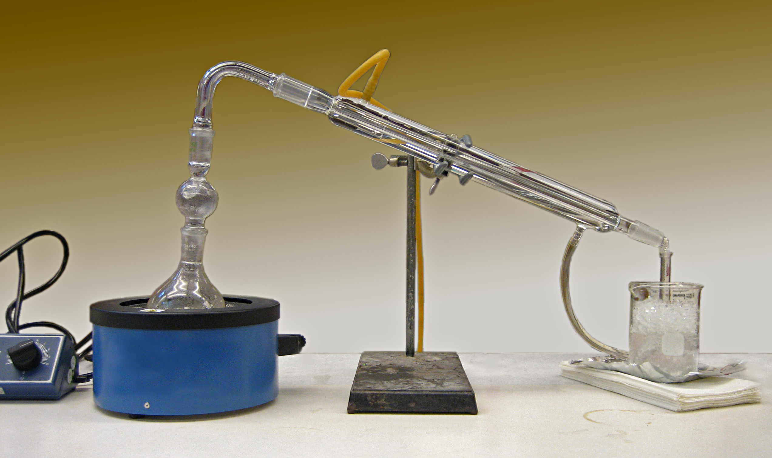
 Then from this we can subtract the triangle !!{0, 10,
20}!! to obtain $${5, 6, 12, 18, 24, 25},$$ a solution to
!!\nk{30}6!! which is not a sum of regular polygons:
Then from this we can subtract the triangle !!{0, 10,
20}!! to obtain $${5, 6, 12, 18, 24, 25},$$ a solution to
!!\nk{30}6!! which is not a sum of regular polygons:


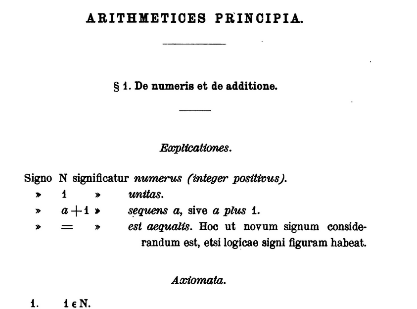
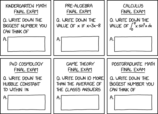


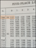
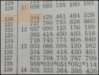
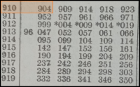
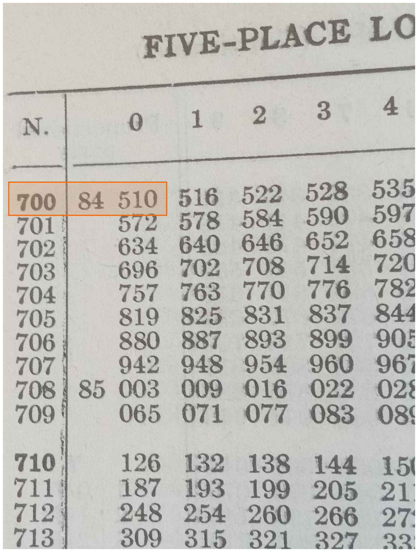
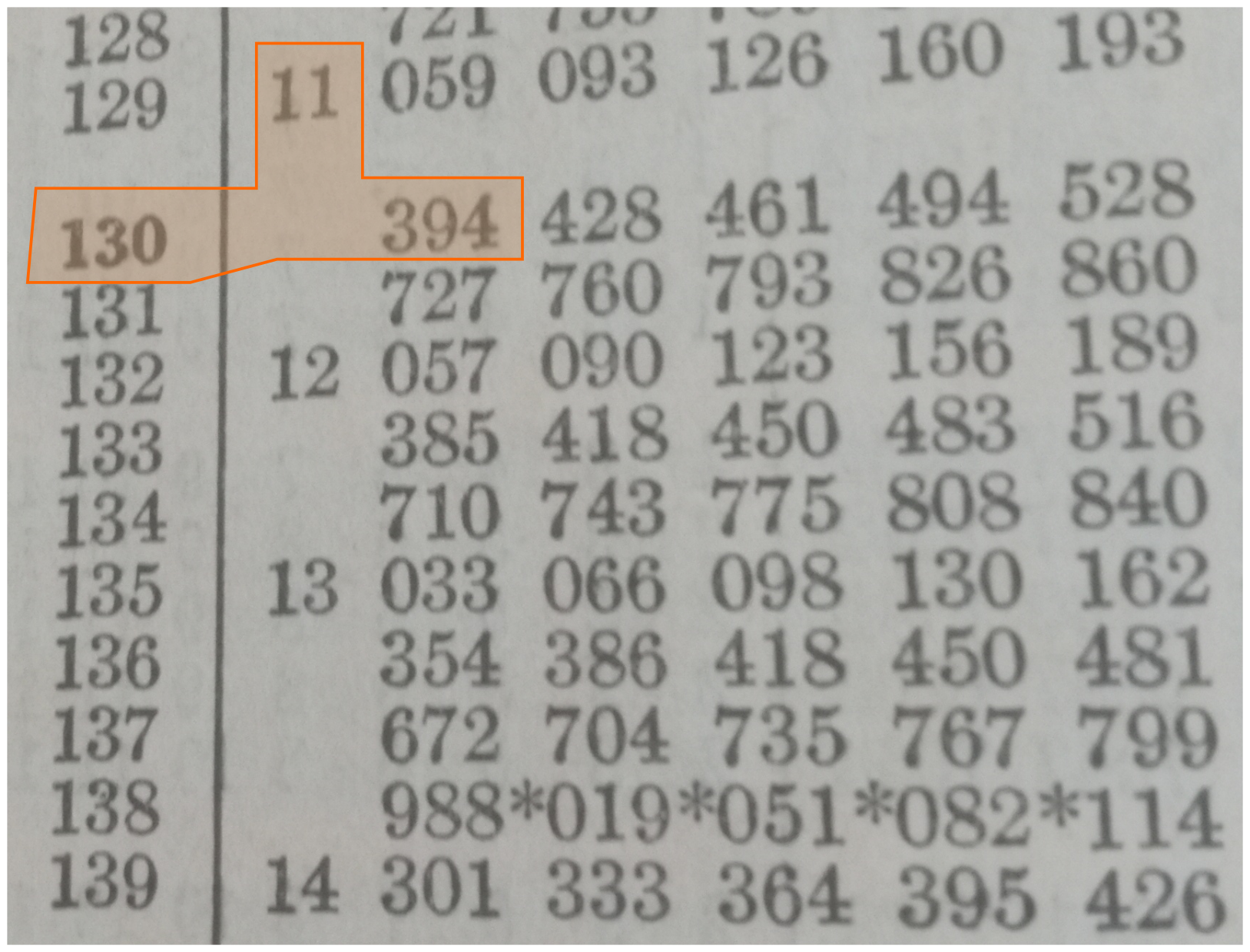
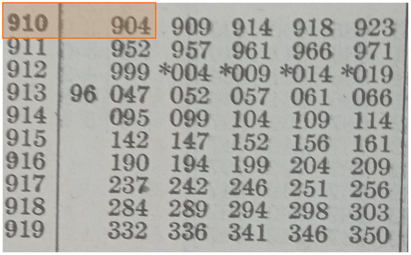
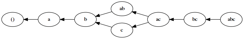
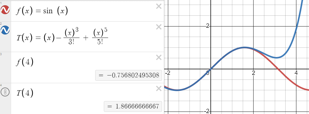
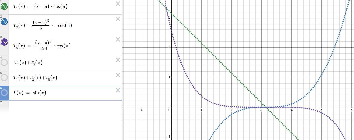
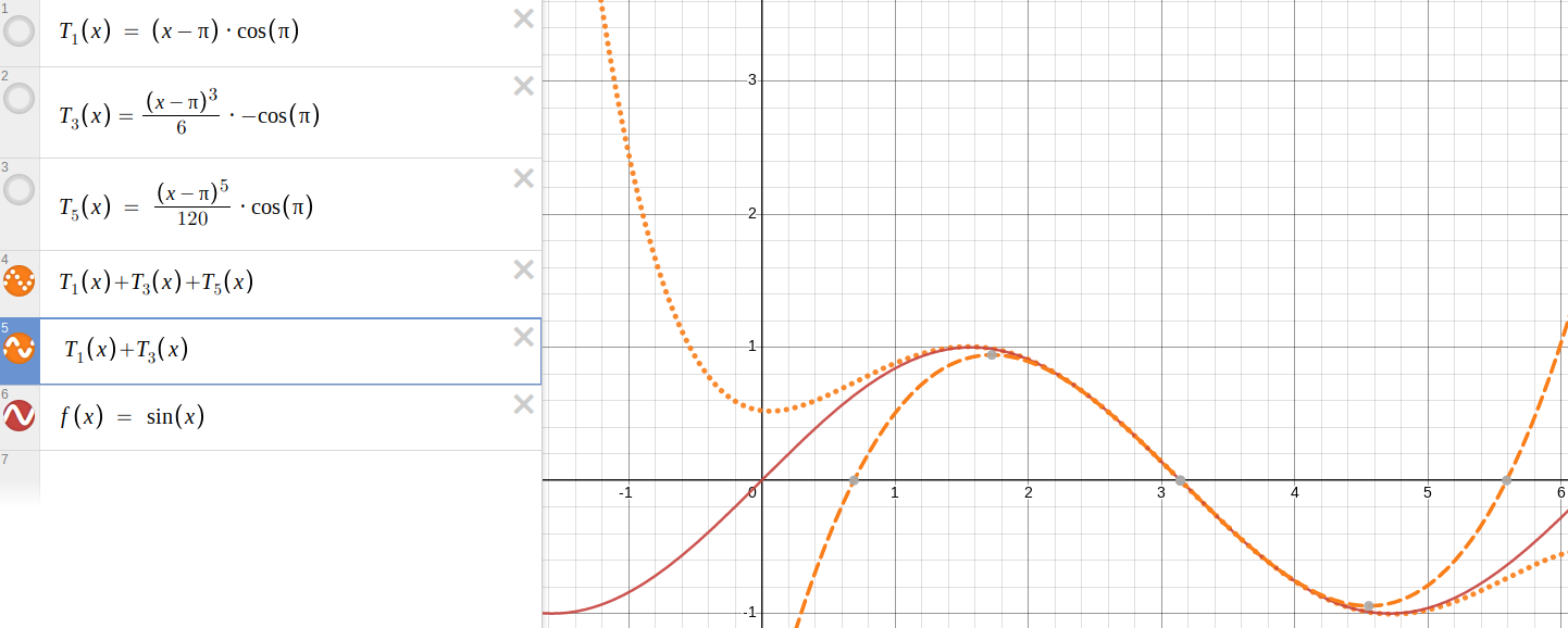
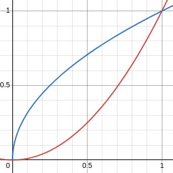
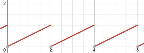


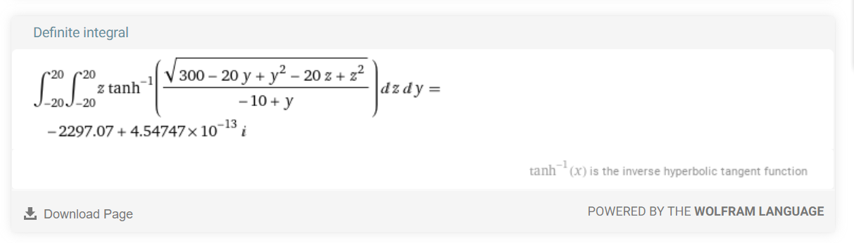
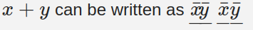
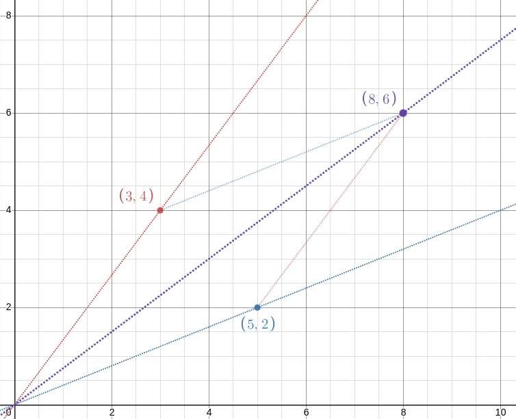
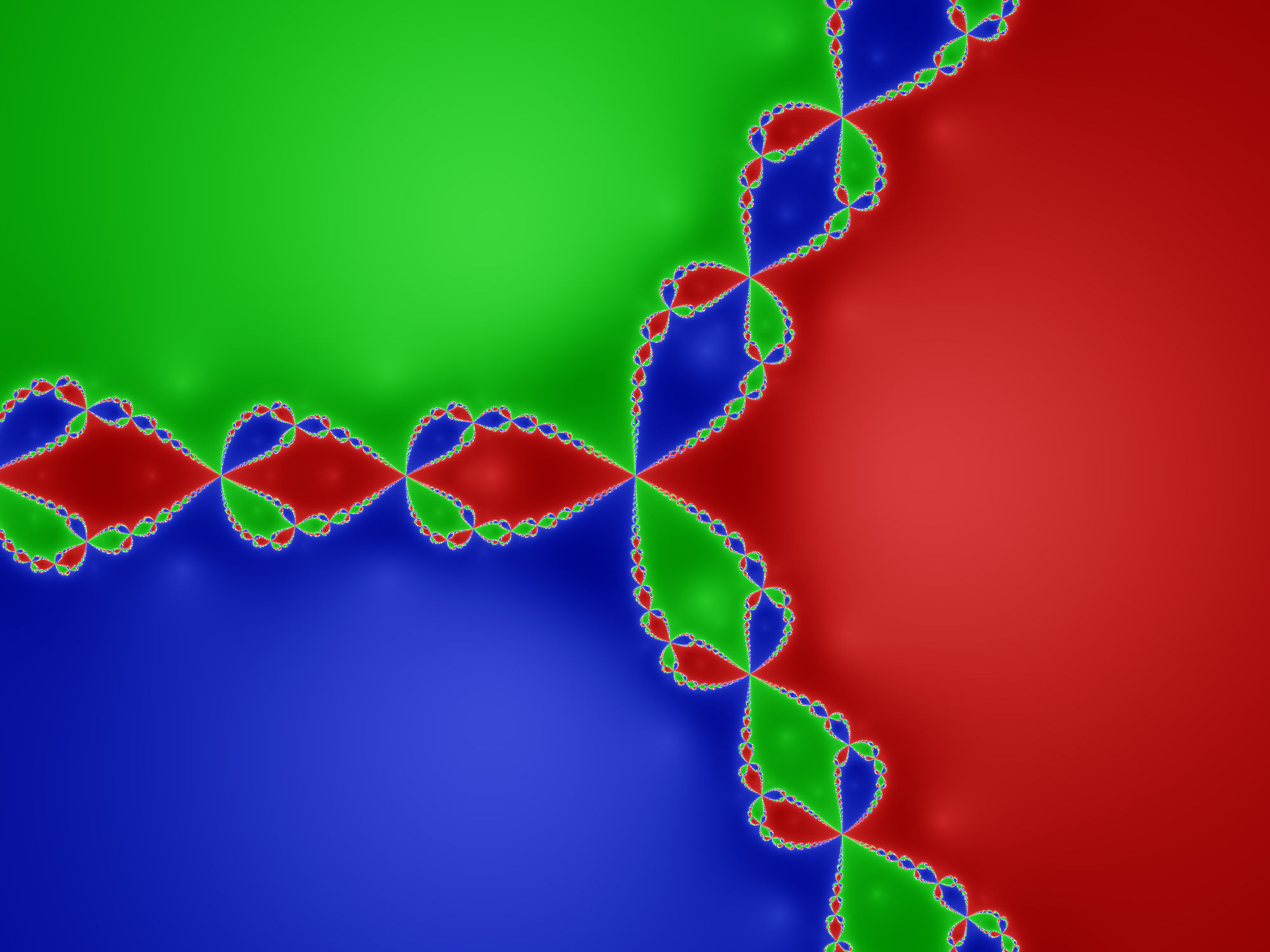
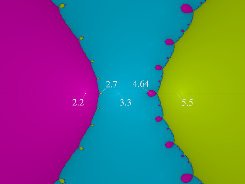
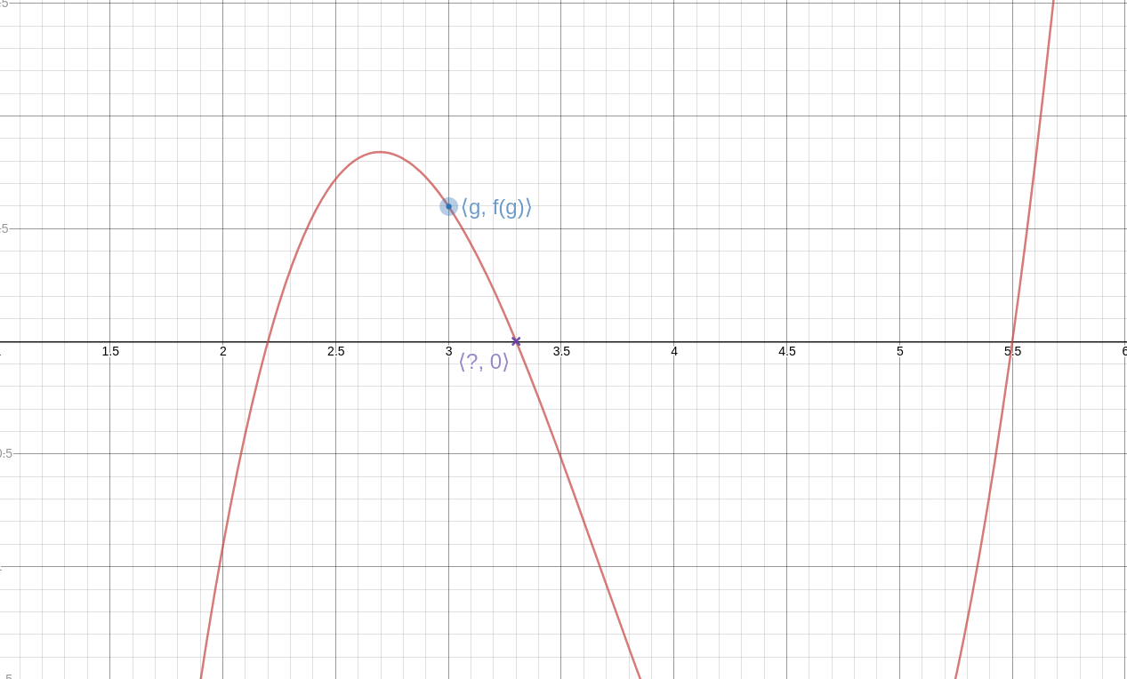
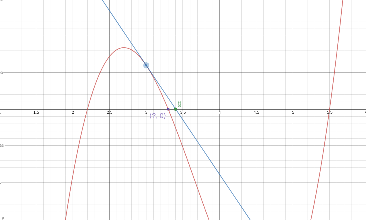
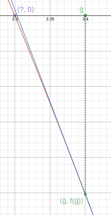


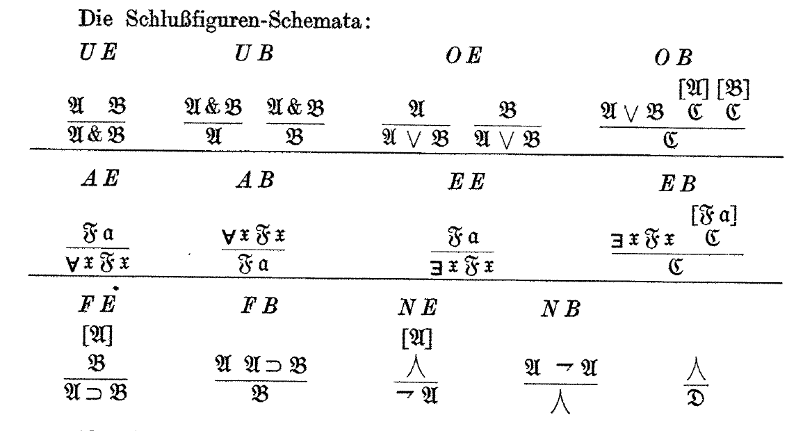


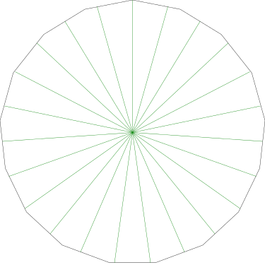
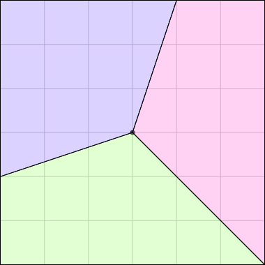 , the central angles deviate from equality by
only a few percent.
, the central angles deviate from equality by
only a few percent.


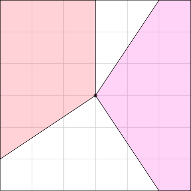
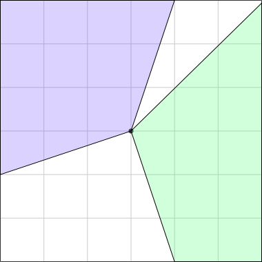
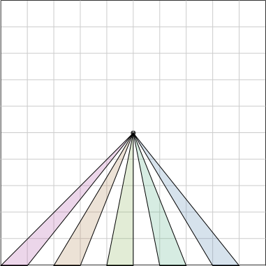
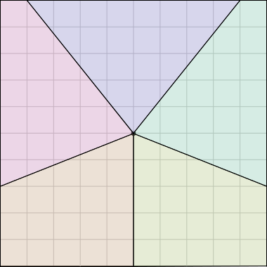

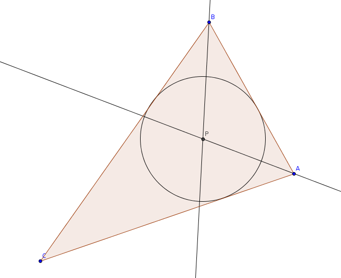
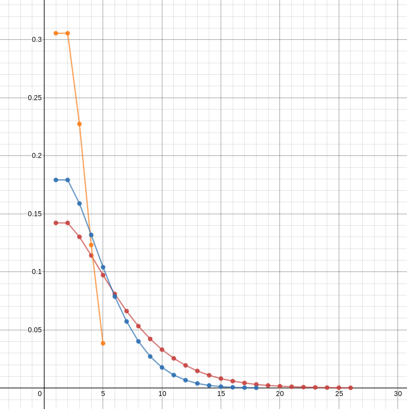
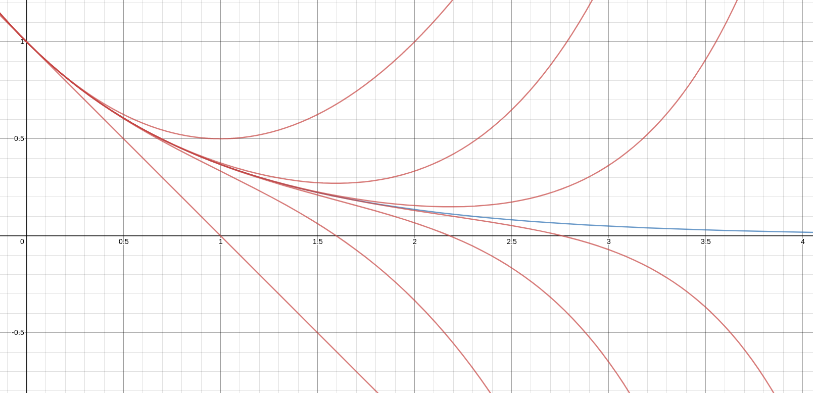


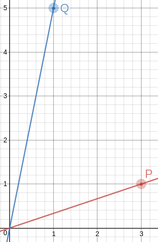
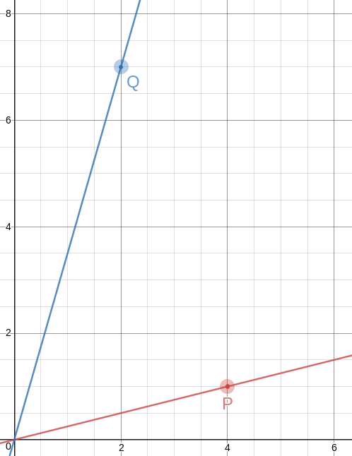
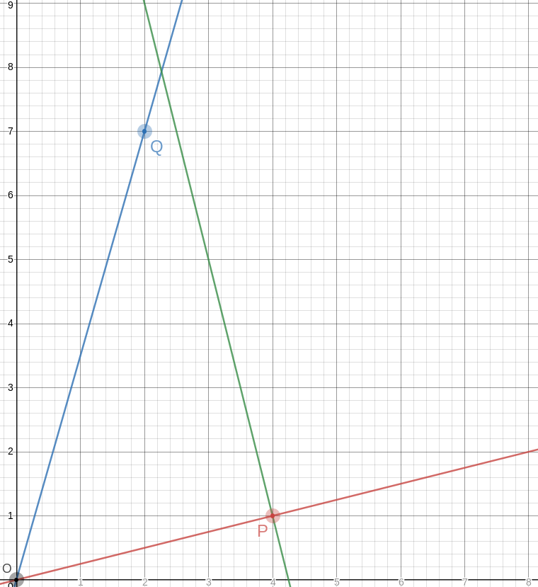
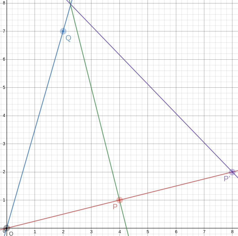


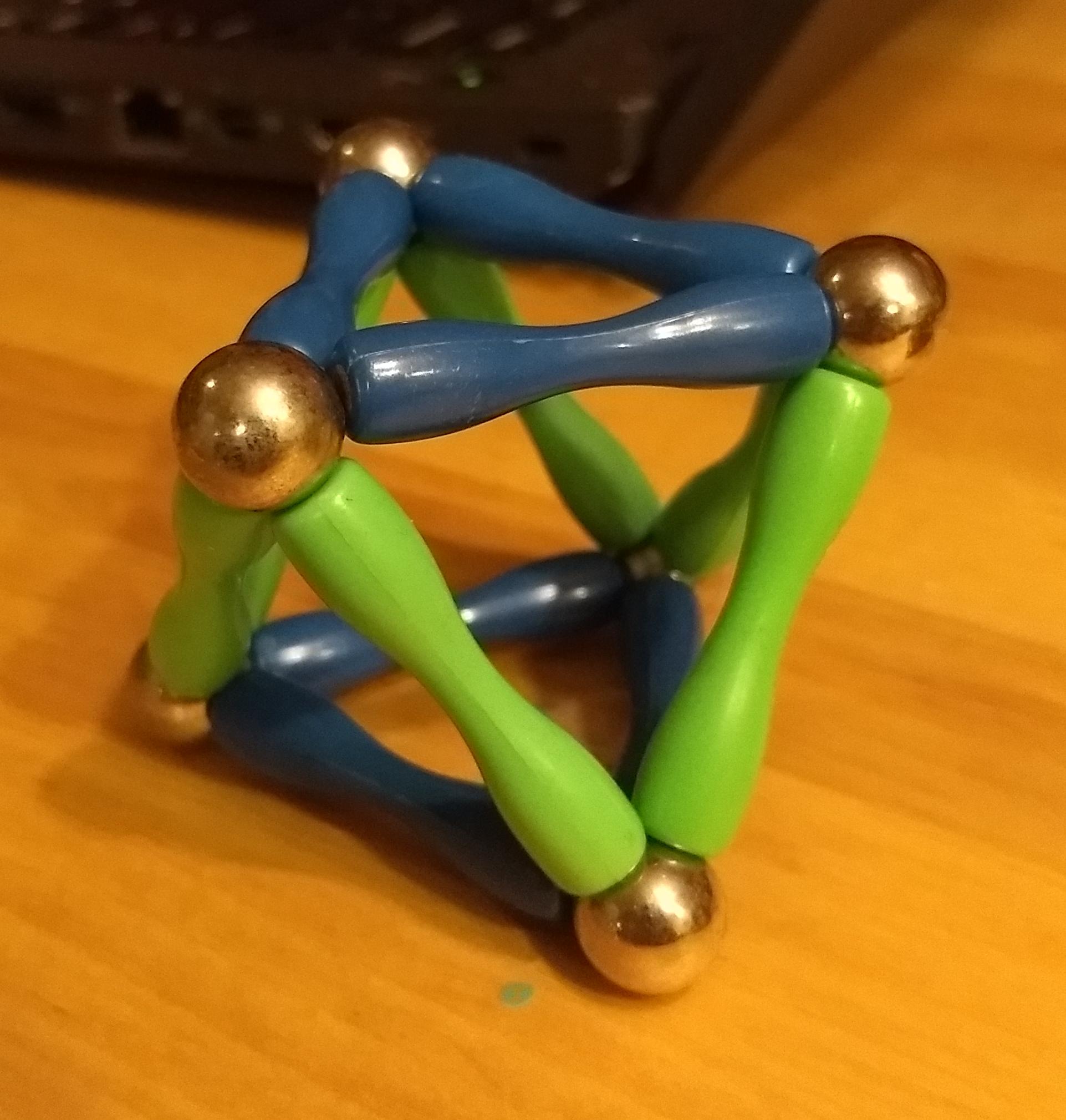
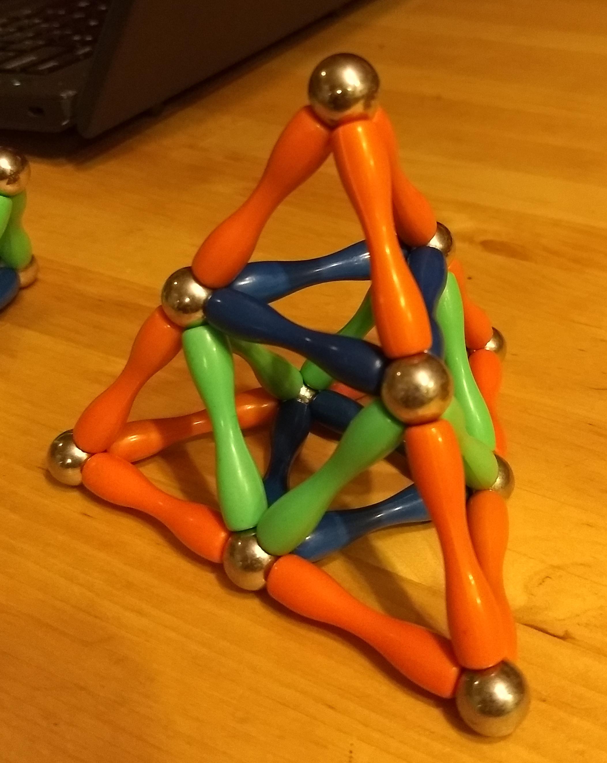
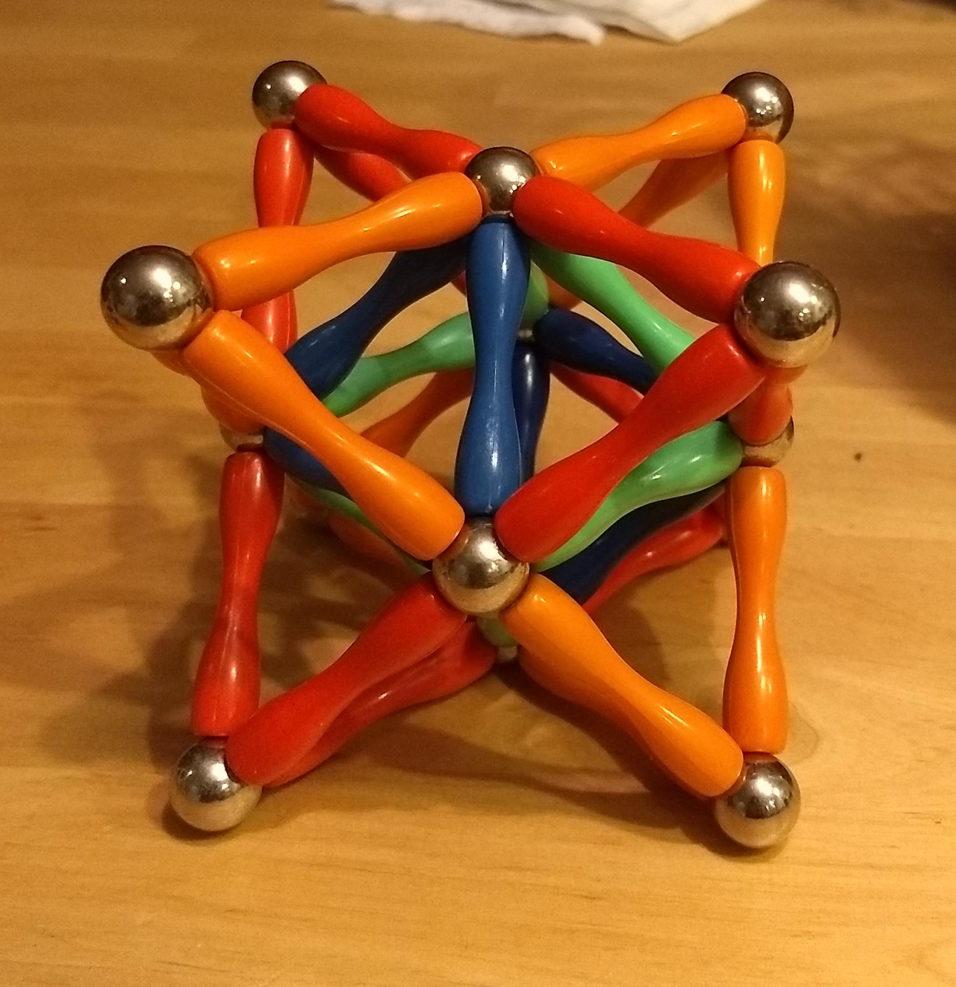


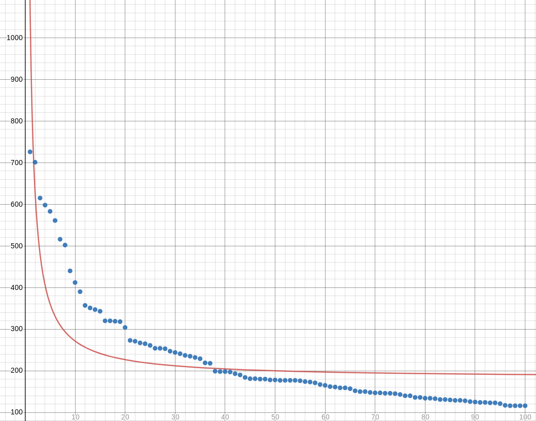


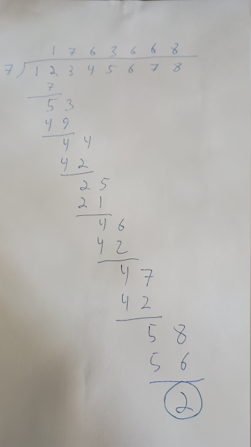
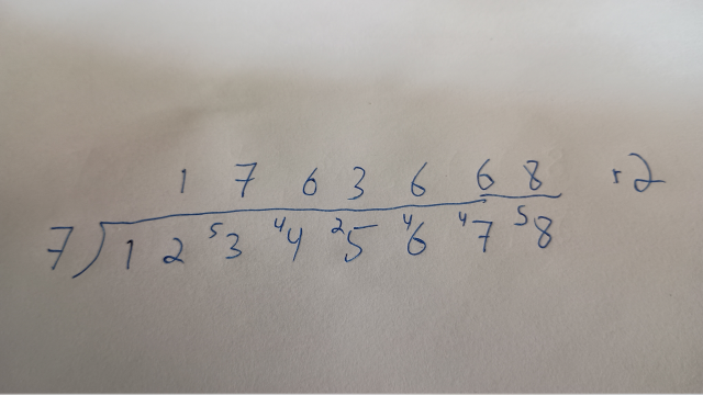

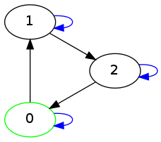
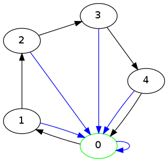
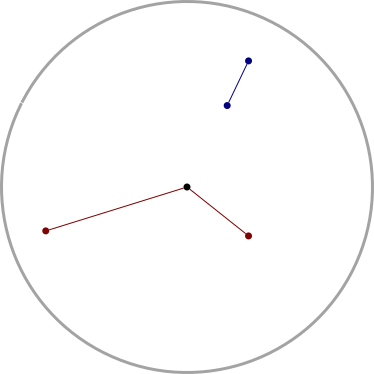

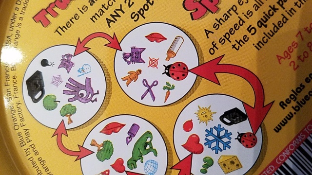

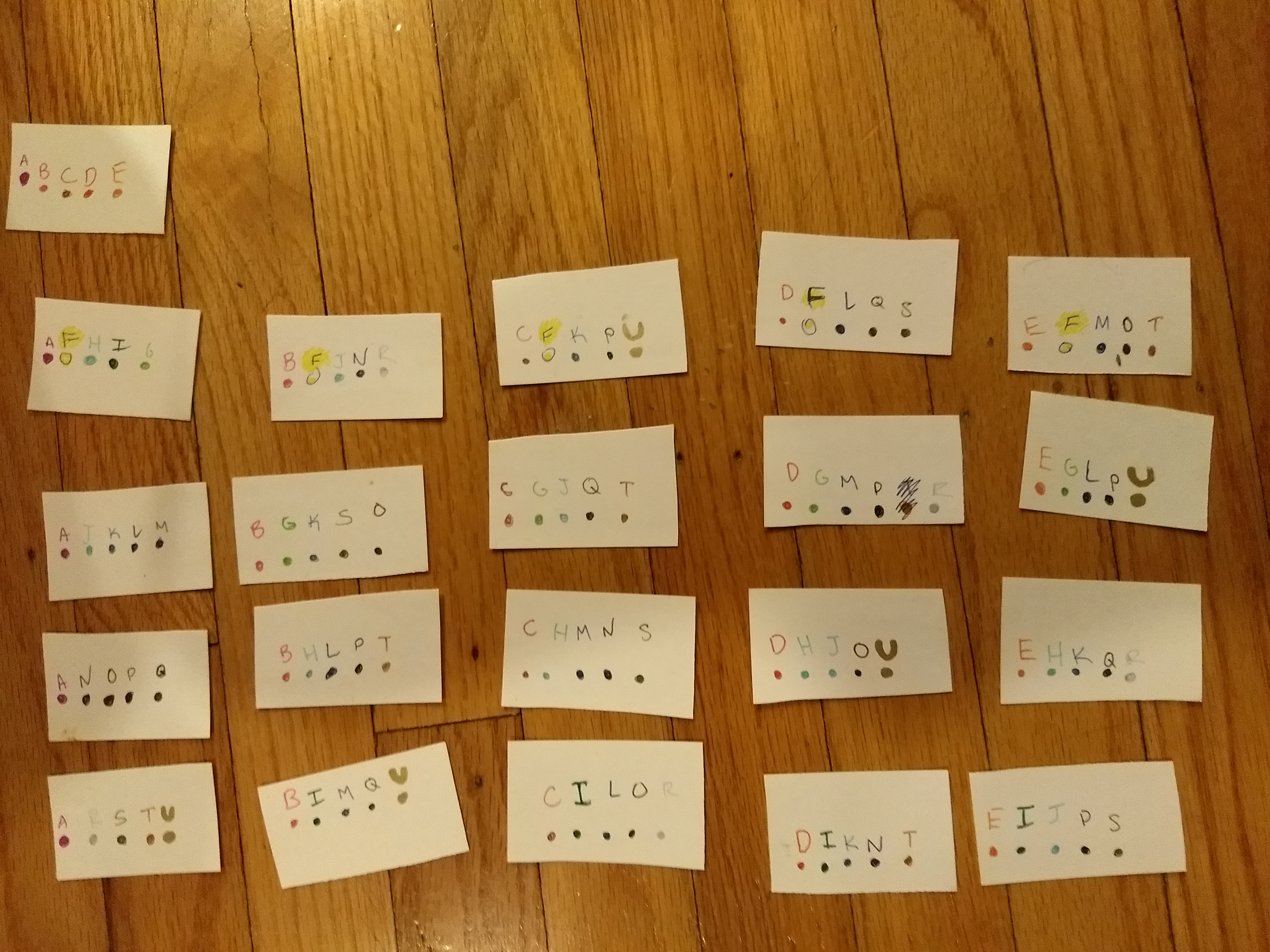
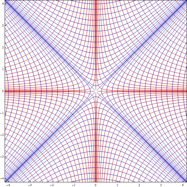 The hyperbolas
!!x^2-y^2 = c!! (in blue) and !!xy=c!! (in red)
The hyperbolas
!!x^2-y^2 = c!! (in blue) and !!xy=c!! (in red)


 represents three vertices, one
in each color. In the picture they are superimposed, but in the actual
graph, no pair of the three is connected by an edge. Instead, each
of the three is connected not to the others but to a tenth vertex that
I omitted from the diagram entirely.
represents three vertices, one
in each color. In the picture they are superimposed, but in the actual
graph, no pair of the three is connected by an edge. Instead, each
of the three is connected not to the others but to a tenth vertex that
I omitted from the diagram entirely.

 and reveal the hidden tenth vertex
and its three edges:
and reveal the hidden tenth vertex
and its three edges:


 and
and  represent single vertices stretched out
into dumbbell shapes. The diagram only shows 14 of the 15 edges; the
fifteenth connects the two dumbbells.
represent single vertices stretched out
into dumbbell shapes. The diagram only shows 14 of the 15 edges; the
fifteenth connects the two dumbbells.


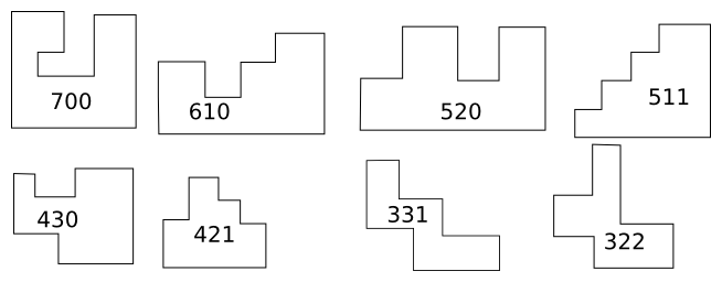
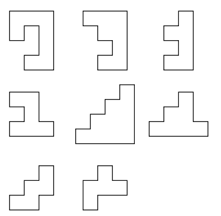

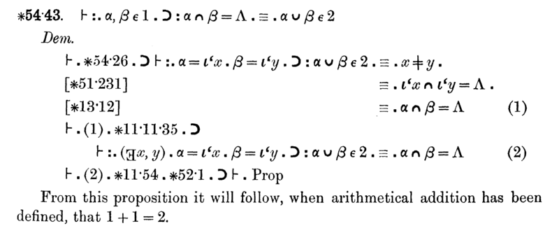


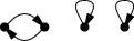
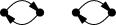
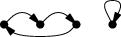
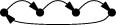

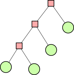


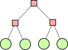
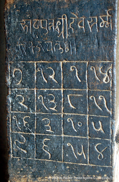


 , and this must be zero. If it were
otherwise, it would appear on its own, as does for example the
, and this must be zero. If it were
otherwise, it would appear on its own, as does for example the
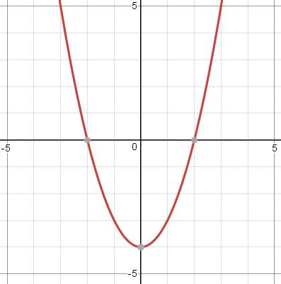
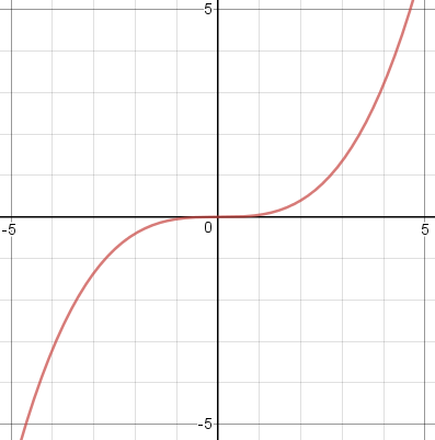
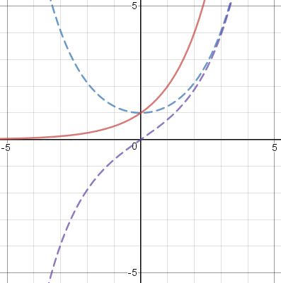
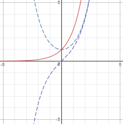
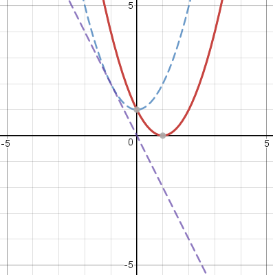
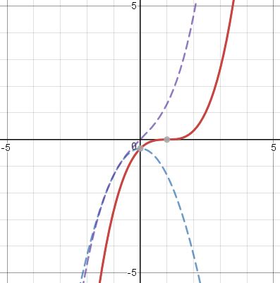
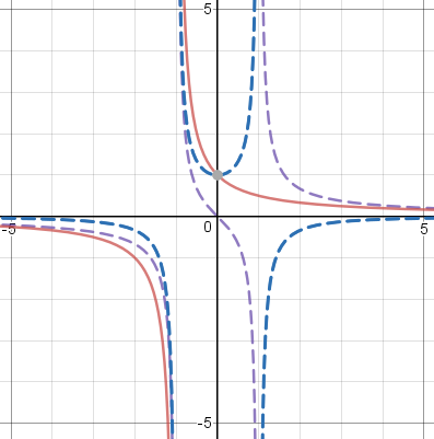
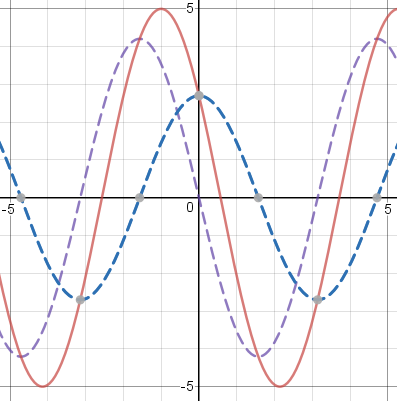
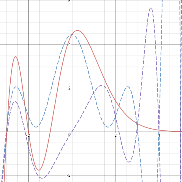
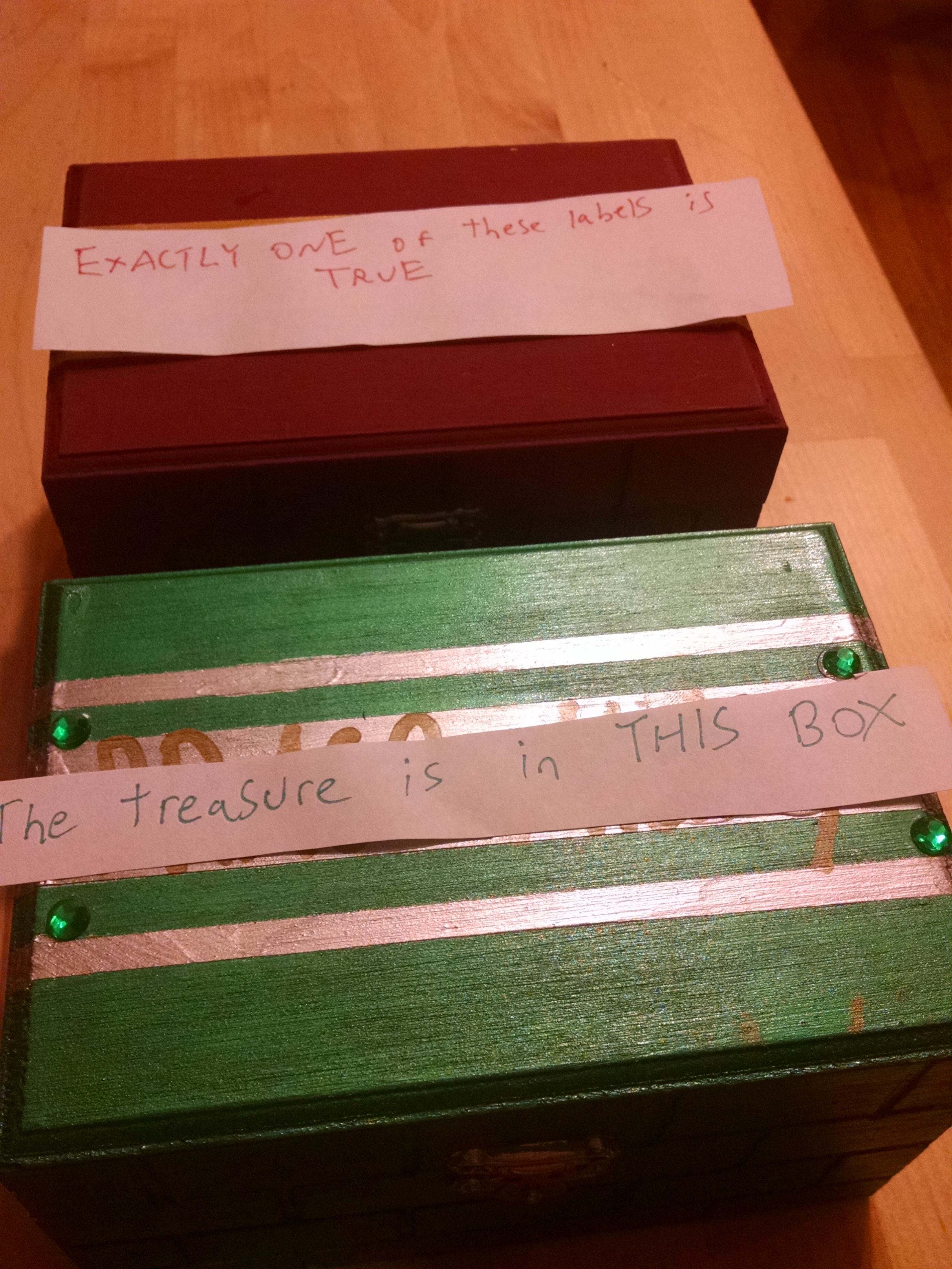
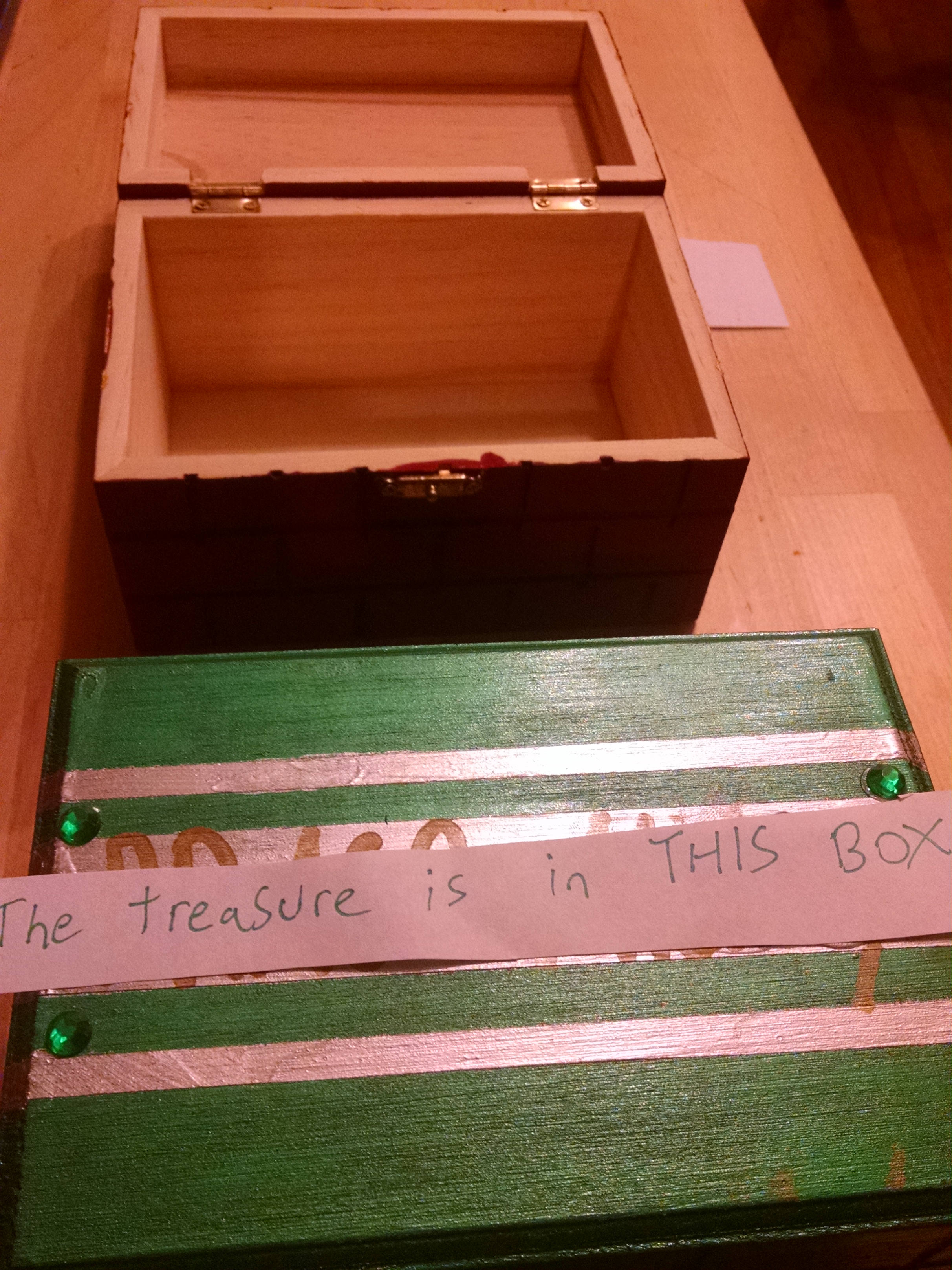
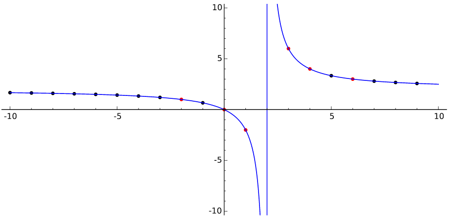
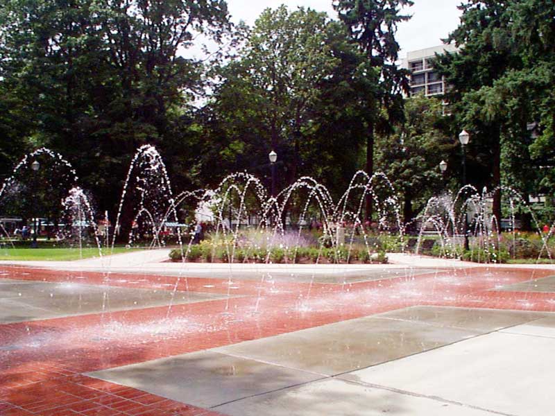
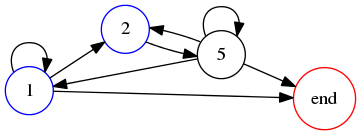
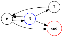
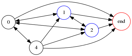
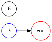
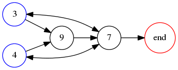
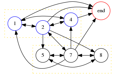

 The term has spawned an
offshoot, the even stranger-sounding "quarter-infinite". This seems
to refer to a geometric object that is unbounded in the same way that
a quarter-plane is unbounded, where "in the same way" is left rather
vague. Consider the set (depicted at left) of all points of the plane
for which 0 ≤ |y/x| ≤ √3, for example; is
this set quarter-infinite, or only 1/6-infinite? Is the set of points
(depicted at right) with xy > 1 and x, y >
0 quarter-infinite? I wouldn't want to say. But the canonical
example is simple: the product of two semi-infinite intervals is a
quarter-infinite set.
The term has spawned an
offshoot, the even stranger-sounding "quarter-infinite". This seems
to refer to a geometric object that is unbounded in the same way that
a quarter-plane is unbounded, where "in the same way" is left rather
vague. Consider the set (depicted at left) of all points of the plane
for which 0 ≤ |y/x| ≤ √3, for example; is
this set quarter-infinite, or only 1/6-infinite? Is the set of points
(depicted at right) with xy > 1 and x, y >
0 quarter-infinite? I wouldn't want to say. But the canonical
example is simple: the product of two semi-infinite intervals is a
quarter-infinite set.


 Last week we took Katara to the pediatrician for a checkup, during which
they weighed, measured, and inoculated her. The measuring device,
which I later learned is called a stadiometer, had a bracket on a slider that went up and down on a
post. Katara stood against the post and the nurse adjusted the bracket
to exactly the top of her head. Then she read off Katara's height from
an attached display.
Last week we took Katara to the pediatrician for a checkup, during which
they weighed, measured, and inoculated her. The measuring device,
which I later learned is called a stadiometer, had a bracket on a slider that went up and down on a
post. Katara stood against the post and the nurse adjusted the bracket
to exactly the top of her head. Then she read off Katara's height from
an attached display. (Click to view the other pictures I took of the post.)
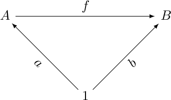

 I forgot to mention in the
original article that I think referring to Gabriel's Horn as
"paradoxical" is straining at a gnat and swallowing a camel.
I forgot to mention in the
original article that I think referring to Gabriel's Horn as
"paradoxical" is straining at a gnat and swallowing a camel.
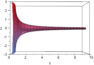
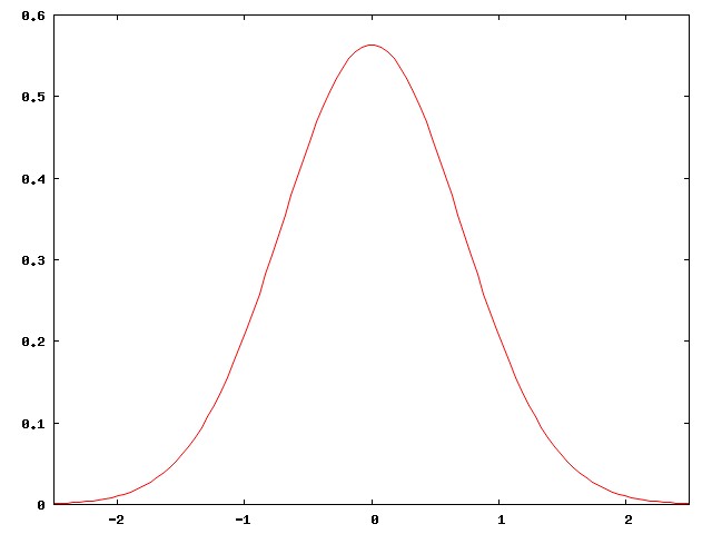
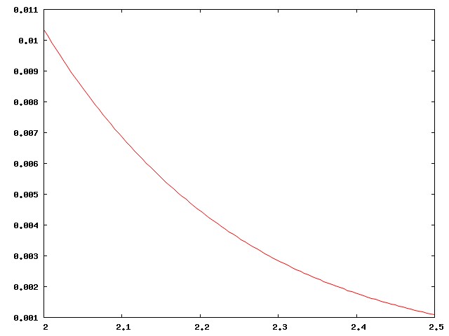
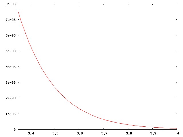
 ,
because then composition of Möbius functions is the same as
multiplication of the corresponding matrices, and so the inverse of a
Möbius function with matrix M is just the function that
corresponds to M-1. Determining whether a set of
Möbius functions is closed under composition is the same as
determining whether the corresponding matrices form a semigroup; you
can figure out what happens when you iterate a Möbius function by
looking at the eigenvalues of M, and so on.
,
because then composition of Möbius functions is the same as
multiplication of the corresponding matrices, and so the inverse of a
Möbius function with matrix M is just the function that
corresponds to M-1. Determining whether a set of
Möbius functions is closed under composition is the same as
determining whether the corresponding matrices form a semigroup; you
can figure out what happens when you iterate a Möbius function by
looking at the eigenvalues of M, and so on. and the matrix
!!{ 2\, 0 \choose 0\,2}!!
are the same Möbius function. So you really need to consider the set
of matrices modulo the equivalence relation that makes two matrices
equivalent if they are the same up to a scalar factor. If you do this
you get a group of matrices called the "projective linear group",
PGL(2). This takes us off into classical group theory and Lie groups,
which I have been intermittently trying to figure out.
and the matrix
!!{ 2\, 0 \choose 0\,2}!!
are the same Möbius function. So you really need to consider the set
of matrices modulo the equivalence relation that makes two matrices
equivalent if they are the same up to a scalar factor. If you do this
you get a group of matrices called the "projective linear group",
PGL(2). This takes us off into classical group theory and Lie groups,
which I have been intermittently trying to figure out.
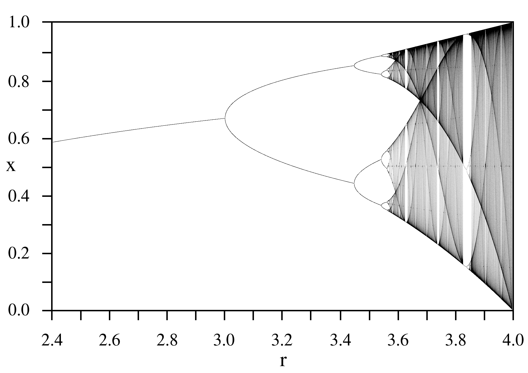

 The instructor was
talking about LC circuits, which are simple circuits with a capacitor
(that's the "C") and an inductor (that's the "L", although I don't
know why). The physics people claim that in such a circuit the
capacitor charges up, and then discharges again, repeatedly. When one
plate of the capacitor is full of electrons, the electrons want to
come out, and equalize the charge on the plates, and so they make a
current flowing from the negative to the positive plate. Without the inductor, the current
would fall off exponentially, as the charge on the plates equalized.
Eventually the two plates would be equally charged and nothing more
would happen.
The instructor was
talking about LC circuits, which are simple circuits with a capacitor
(that's the "C") and an inductor (that's the "L", although I don't
know why). The physics people claim that in such a circuit the
capacitor charges up, and then discharges again, repeatedly. When one
plate of the capacitor is full of electrons, the electrons want to
come out, and equalize the charge on the plates, and so they make a
current flowing from the negative to the positive plate. Without the inductor, the current
would fall off exponentially, as the charge on the plates equalized.
Eventually the two plates would be equally charged and nothing more
would happen. A pink square means that the polynomials are relatively prime; a white square
means that they are not.
Another version of this table appeared on the cover of
Mathematics Magazine. It's shown at right.
A pink square means that the polynomials are relatively prime; a white square
means that they are not.
Another version of this table appeared on the cover of
Mathematics Magazine. It's shown at right.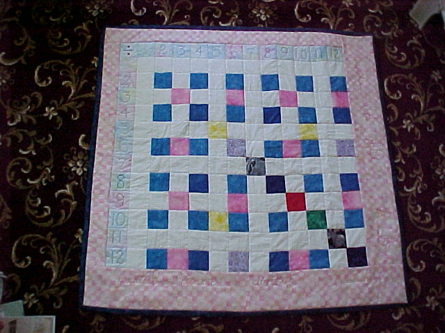

 On Thursday I didn't know what went wrong with (2,2,2); it seemed
fine. (I found it a little challenging to embed it in the plane, but
I'm not sure if it would still be challenging if it hadn't been the
middle of the night.) I decided that when I got into the office on
Friday I would try making a model of it with my magnet toy and see
what happened.
On Thursday I didn't know what went wrong with (2,2,2); it seemed
fine. (I found it a little challenging to embed it in the plane, but
I'm not sure if it would still be challenging if it hadn't been the
middle of the night.) I decided that when I got into the office on
Friday I would try making a model of it with my magnet toy and see
what happened. (2,0,6) was a planar graph too, and so the problem had to be
geometric, not topological. When I got to the office, I put it
together. It also worked fine, but the result is not a polyhedron.
The thing you get could be described as a gyroelongated triangular
dipyramid. That is, you take an octahedron and glue tetrahedra to two
of its opposite faces. But then the faces of the tetrahedra are
coplanar with the faces of the octahedron to which they abut, and this
is forbidden in polyhedra. When that happens you're supposed to
eliminate the intervening edge and consider the two faces to be a
single face, a rhombus in this case.
(2,0,6) was a planar graph too, and so the problem had to be
geometric, not topological. When I got to the office, I put it
together. It also worked fine, but the result is not a polyhedron.
The thing you get could be described as a gyroelongated triangular
dipyramid. That is, you take an octahedron and glue tetrahedra to two
of its opposite faces. But then the faces of the tetrahedra are
coplanar with the faces of the octahedron to which they abut, and this
is forbidden in polyhedra. When that happens you're supposed to
eliminate the intervening edge and consider the two faces to be a
single face, a rhombus in this case.
 The resulting thing is not a
polyhedron with 12 triangular faces, but one with six rhombic faces (a
rhombohedron), essentially a squashed cube. In fact, it's exactly
what you get if you make a cube from the magnet toy and then try to
insert another unit-length rod into the diagonal of each of the six
faces. You have to squash the cube to do this, of course, since the
diagonals had length √2 before and length 1 after.
The resulting thing is not a
polyhedron with 12 triangular faces, but one with six rhombic faces (a
rhombohedron), essentially a squashed cube. In fact, it's exactly
what you get if you make a cube from the magnet toy and then try to
insert another unit-length rod into the diagonal of each of the six
faces. You have to squash the cube to do this, of course, since the
diagonals had length √2 before and length 1 after.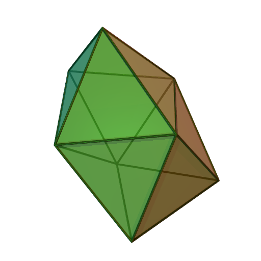 The snub
disphenoid is pictured at left. I do not know why it is called that,
and I ought to know, because I am the principal author (so far) of the
Wikipedia article on the disphenoid. Also,
I never quite figured out what "snub" means in this context, despite
perusing that section of H.S.M. Coxeter's book on polytopes at some
length. It has something to do with being halfway between what you
get when you cut all the corners off, and what you get when you cut all
the corners off again.
The snub
disphenoid is pictured at left. I do not know why it is called that,
and I ought to know, because I am the principal author (so far) of the
Wikipedia article on the disphenoid. Also,
I never quite figured out what "snub" means in this context, despite
perusing that section of H.S.M. Coxeter's book on polytopes at some
length. It has something to do with being halfway between what you
get when you cut all the corners off, and what you get when you cut all
the corners off again.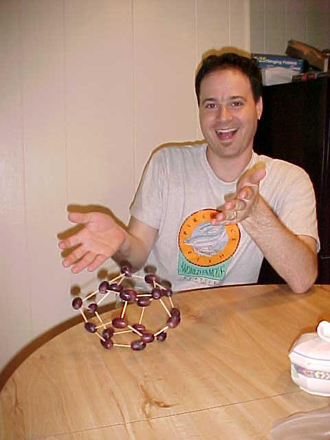
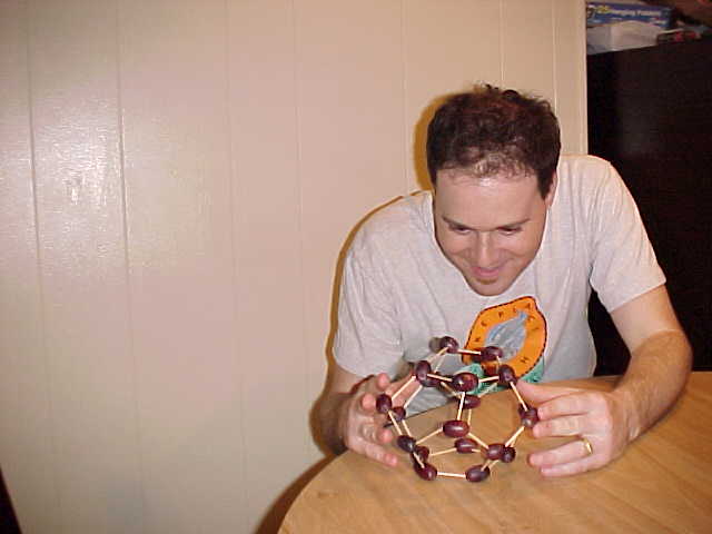 Anyway, earlier this week I was visiting John Batzel, who works
upstairs from me, and discovered that he had obtained a really cool
toy. It was a collection of large steel ball bearings and colored
magnetic rods, which could be assembled into various polyhedra and
trusses. This is irresistible to me. The pictures at right, taken around
2002, show me modeling a dodecahedron with less suitable
materials.
Anyway, earlier this week I was visiting John Batzel, who works
upstairs from me, and discovered that he had obtained a really cool
toy. It was a collection of large steel ball bearings and colored
magnetic rods, which could be assembled into various polyhedra and
trusses. This is irresistible to me. The pictures at right, taken around
2002, show me modeling a dodecahedron with less suitable
materials.
 Another is the icosahedron. Imagine making a belt of 10 triangles,
alternating up and down, and then connect the ends of the belt. The result is a
shape called a pentagonal
antiprism, shown at left. The edges of the down-pointing triangles form a
pentagon on the top of the antiprism, and the edges of the up-pointing
triangles form one on the bottom. Attach a pentagonal pyramid to each
of these pentagons, and you have an icosahedron, with a total of 20
faces.
Another is the icosahedron. Imagine making a belt of 10 triangles,
alternating up and down, and then connect the ends of the belt. The result is a
shape called a pentagonal
antiprism, shown at left. The edges of the down-pointing triangles form a
pentagon on the top of the antiprism, and the edges of the up-pointing
triangles form one on the bottom. Attach a pentagonal pyramid to each
of these pentagons, and you have an icosahedron, with a total of 20
faces. for example. The algorithm, as I wrote
it, calculates intermediate values 8, 8, 56, 28, 168, 56, 280, 70, and
70 is the final answer. If your computer has 7-bit machine integers,
the answer (70) will fit, but the calculation will overflow along the
way at the 168 and 280 steps.
for example. The algorithm, as I wrote
it, calculates intermediate values 8, 8, 56, 28, 168, 56, 280, 70, and
70 is the final answer. If your computer has 7-bit machine integers,
the answer (70) will fit, but the calculation will overflow along the
way at the 168 and 280 steps. . For example, instead of calculating !!100\choose98!!, calculate
  . I didn't mention this in the original article
because it was irrelevant to the main point, and because I thought it
was obvious.
. I didn't mention this in the original article
because it was irrelevant to the main point, and because I thought it
was obvious. is to use the following recurrence:
 would force it to be
4th-degree.
would force it to be
4th-degree.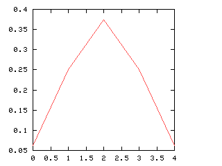
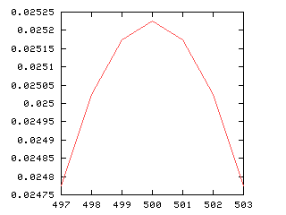
 in the denominator, with the result that
distributions with a lot of equal-sized parts tend to appear less
frequently than you might otherwise expect.
in the denominator, with the result that
distributions with a lot of equal-sized parts tend to appear less
frequently than you might otherwise expect. 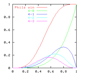
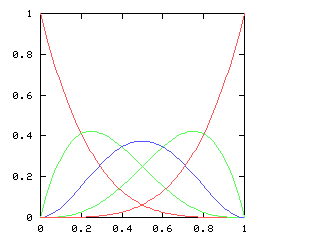
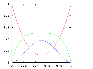
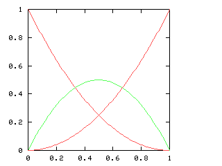
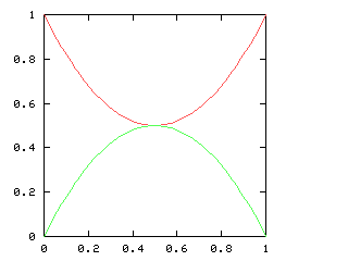

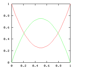
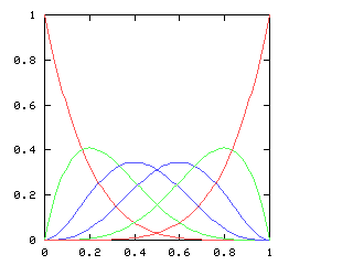
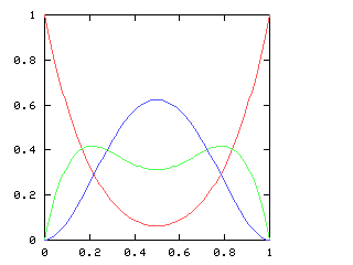
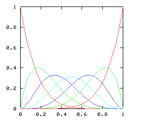


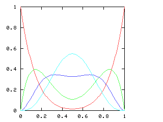

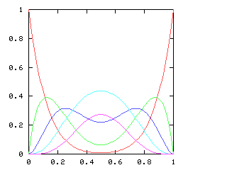
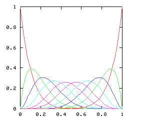
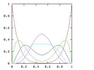
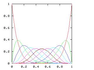
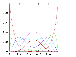
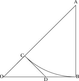
 denotes the so-called multinomial
coefficient, equal to !!{N!\over
p_1!p_2!\ldots p_k!}!!.
denotes the so-called multinomial
coefficient, equal to !!{N!\over
p_1!p_2!\ldots p_k!}!!. in terms of the ni:
 does not involve S, we can easily
precalculate it for some pattern and then plug it into the rest of the
formula to get the likelihood of rolling that pattern with different
kinds of dice. For example, consider the two-pairs pattern AABBC.
This pattern has n1 = 1,
n2 = 2, so the key factor comes out to be 15.
Plugging this into the rest of the formula, we see that the probability of
rolling AABBC with five S-sided dice is
!!90 {S \choose 3} S^{-5}!!.
Here is a tabulation:
does not involve S, we can easily
precalculate it for some pattern and then plug it into the rest of the
formula to get the likelihood of rolling that pattern with different
kinds of dice. For example, consider the two-pairs pattern AABBC.
This pattern has n1 = 1,
n2 = 2, so the key factor comes out to be 15.
Plugging this into the rest of the formula, we see that the probability of
rolling AABBC with five S-sided dice is
!!90 {S \choose 3} S^{-5}!!.
Here is a tabulation: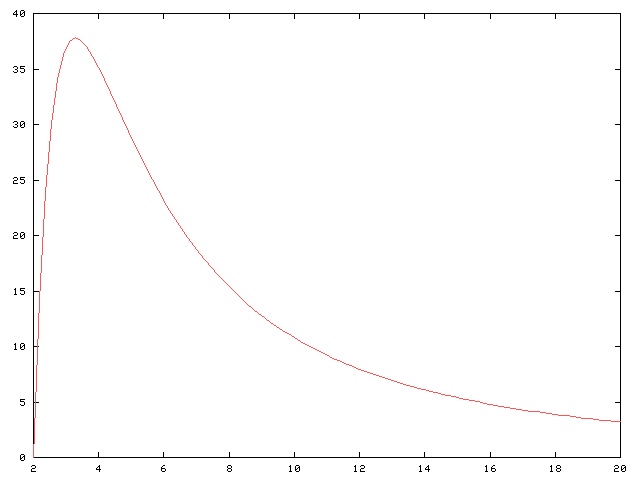
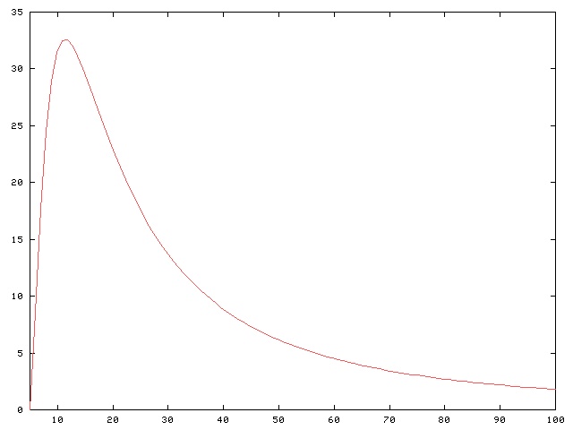
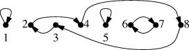


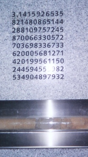

 , just go away, because we
already proved them for sets and relations are sets. The null
relation is the null set. The universal relation is
the universal set.
, just go away, because we
already proved them for sets and relations are sets. The null
relation is the null set. The universal relation is
the universal set.


 is the ultimate source of the use of the word
lambda to denote an anonymous function in the Lisp and Python
programming languages. I am sure you know that these languages get
"lambda" from the use of the Greek letter λ by Alonzo Church to
represent function abstraction in his "λ-calculus": In Lisp,
(lambda (u) B) is a function that takes an argument
u and returns the value of B; in the λ-calculus,
λu.B is a function that takes an argument
u and returns the value of B. (Recall also that
Church was the doctoral advisor of John McCarthy, the inventor of Lisp.)
Norvig says that Church
was originally planning to write the function
λu.B as û.B, but his printer
could not do circumflex accents. So he considered moving the
circumflex to the left and using a capital lambda instead:
Λu.B. The capital Λ looked too much like
logical and ∧, which was confusing, so he used lowercase lambda
λ instead.
is the ultimate source of the use of the word
lambda to denote an anonymous function in the Lisp and Python
programming languages. I am sure you know that these languages get
"lambda" from the use of the Greek letter λ by Alonzo Church to
represent function abstraction in his "λ-calculus": In Lisp,
(lambda (u) B) is a function that takes an argument
u and returns the value of B; in the λ-calculus,
λu.B is a function that takes an argument
u and returns the value of B. (Recall also that
Church was the doctoral advisor of John McCarthy, the inventor of Lisp.)
Norvig says that Church
was originally planning to write the function
λu.B as û.B, but his printer
could not do circumflex accents. So he considered moving the
circumflex to the left and using a capital lambda instead:
Λu.B. The capital Λ looked too much like
logical and ∧, which was confusing, so he used lowercase lambda
λ instead.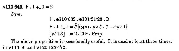


 What about turning the squares over? Are the two squares to the right
"the same"?
Let's say that the squares are inked
on only one side, so that those two would not considered the
same, even if we decided to allow squares with green wedges. Later on
we will make the decision the other way and see how things change.
What about turning the squares over? Are the two squares to the right
"the same"?
Let's say that the squares are inked
on only one side, so that those two would not considered the
same, even if we decided to allow squares with green wedges. Later on
we will make the decision the other way and see how things change.

 OK, so let's see. All four wedges might be the same color, and
there are 3 colors, so there are 3 ways to do that, shown at right.
OK, so let's see. All four wedges might be the same color, and
there are 3 colors, so there are 3 ways to do that, shown at right.


 Or there might only be two colors. In
that case, there might be three wedges of one color and one of
another, there are 6 ways to do that, depending on how we pick the
colors; these six are shown at right.
Or there might only be two colors. In
that case, there might be three wedges of one color and one of
another, there are 6 ways to do that, depending on how we pick the
colors; these six are shown at right.


 If we use all three colors, then two wedges are in one of the colors,
and one wedge in each of the other two colors. The two wedges of the
same color might be adjacent to each other or opposite. In either case, we have three choices for the color of the two wedges that are
the same, after which the colors of the other two wedges are forced.
So that's 3 colorings with two adjacent wedges the same color:
If we use all three colors, then two wedges are in one of the colors,
and one wedge in each of the other two colors. The two wedges of the
same color might be adjacent to each other or opposite. In either case, we have three choices for the color of the two wedges that are
the same, after which the colors of the other two wedges are forced.
So that's 3 colorings with two adjacent wedges the same color:

 And 3 colorings with two opposite wedges the same color:


 and
and
 were the same because differences
of a simple rotation didn't count? Well, the first thing you do is
you make a list of all the kinds of motions that "don't
count". In this case, there are four motions:
were the same because differences
of a simple rotation didn't count? Well, the first thing you do is
you make a list of all the kinds of motions that "don't
count". In this case, there are four motions:


 , we allow only one, since they are
now considered "the same". There are three such pairs, so this
reduces our count by exactly 3.
, we allow only one, since they are
now considered "the same". There are three such pairs, so this
reduces our count by exactly 3.

 and
and  are considered the same) there are
51 colorings.
are considered the same) there are
51 colorings.  is actually a letter
"S", chosen by Leibnitz because it was the first letter of the word
"sum". Seth David Schoen suggested that Leibnitz probably wrote in
Latin, so that it is actually the first letter of the word "summa",
which means "sum" in Latin. I do not know, but I will see if I can
track down the original paper.
is actually a letter
"S", chosen by Leibnitz because it was the first letter of the word
"sum". Seth David Schoen suggested that Leibnitz probably wrote in
Latin, so that it is actually the first letter of the word "summa",
which means "sum" in Latin. I do not know, but I will see if I can
track down the original paper. 


 1.
The most obviously germane fact I came up with was this:
Inscribe a regular hexagon in the unit circle. Such a hexagon
obviously has a perimeter of 6. The circle goes through the same six
points, but instead of taking direct paths between them, it takes a
circuitous route, so its perimeter is a bit more than 6.
Therefore pi is a bit more than 3.
1.
The most obviously germane fact I came up with was this:
Inscribe a regular hexagon in the unit circle. Such a hexagon
obviously has a perimeter of 6. The circle goes through the same six
points, but instead of taking direct paths between them, it takes a
circuitous route, so its perimeter is a bit more than 6.
Therefore pi is a bit more than 3.
 The next item is my second favorite, after the
observation about the inscribed hexagon:
The next item is my second favorite, after the
observation about the inscribed hexagon:
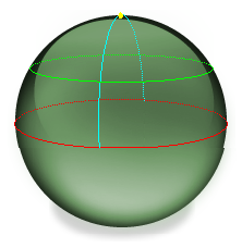 The "diameter" of a circle is the longest possible "line" you can draw
from one point on the circle to another. A diameter of a circle has
the property that it always goes through the center of the circle, as
you would hope and expect. For the equator, a diameter goes through
the north pole. The picture to the right shows the equator in red,
its center, the north pole, in yellow, and a diameter of the equator
in blue. The 49th parallel is in green.
The "diameter" of a circle is the longest possible "line" you can draw
from one point on the circle to another. A diameter of a circle has
the property that it always goes through the center of the circle, as
you would hope and expect. For the equator, a diameter goes through
the north pole. The picture to the right shows the equator in red,
its center, the north pole, in yellow, and a diameter of the equator
in blue. The 49th parallel is in green.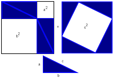


;

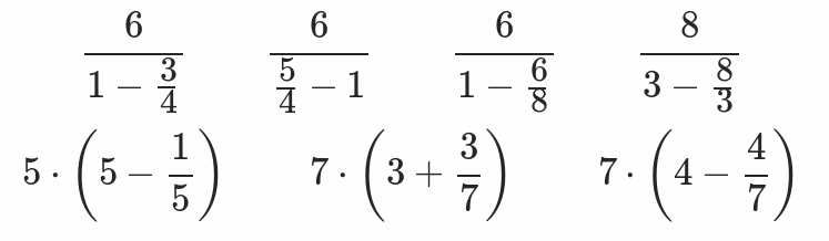