The Universe of Discourse

Sun, 18 Oct 2020

While messing around with Newton's method for last week's article, I built this Desmos thingy:

The red point represents the initial guess; grab it and drag it around, and watch how the later iterations change. Or, better, visit the Desmos site and play with the slider yourself.

(The curve here is !!y = (x-2.2)(x-3.3)(x-5.5)!!; it has a local maximum at around !!2.7!!, and a local minimum at around !!4.64!!.)

Watching the attractor point jump around I realized I was arriving at a much better understanding of the instability of the convergence. Clearly, if your initial guess happens to be near an extremum of !!f!!, the next guess could be arbitrarily far away, rather than a small refinement of the original guess. But even if the original guess is pretty good, the refinement might be near an extremum, and then the following guess will be somewhere random. For example, although !!f!! is quite well-behaved in the interval !![4.3, 4.35]!!, as the initial guess !!g!! increases across this interval, the refined guess !!\hat g!! decreases from !!2.74!! to !!2.52!!, and in between these there is a local maximum that kicks the ball into the weeds. The result is that at !!g=4.3!! the method converges to the largest of the three roots, and at !!g=4.35!!, it converges to the smallest.

This is where the Newton basins come from:

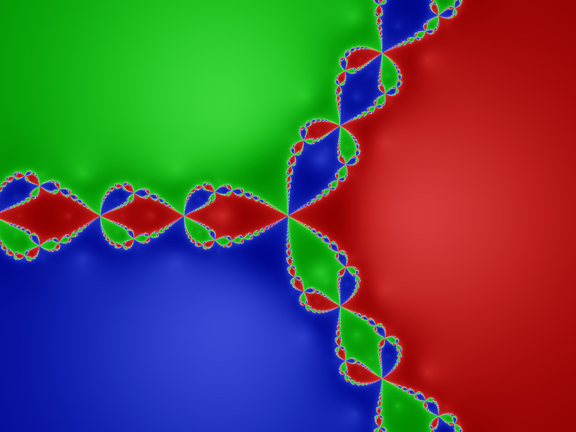
$Julia set for the rational function associated to Newton's method for ƒ:z→z³−1. The plane is divided symmetrically into three regions, colored red, green, and blue. The boundary of each two regions (red and green, say) is inhabited by a series of leaf shapes of the third color (blue), and the boundaries between the main regions (green, say) and the (blue) leaves are inhabited by smaller leaves again of the other color (red), and so on ad infinitum. The boundaries are therefore an infinitely detailed filigree of smaller and smaller leaves of all three colors.$

Here we are considering the function !!f:z\mapsto z^3 -1!! in the complex plane. Zero is at the center, and the obvious root, !!z=1!! is to its right, deep in the large red region. The other two roots are at the corresponding positions in the green and blue regions.

Starting at any red point converges to the !!z=1!! root. Usually, if you start near this root, you will converge to it, which is why all the points near it are red. But some nearish starting points are near an extremum, so that the next guess goes wild, and then the iteration ends up at the green or the blue root instead; these areas are the rows of green and blue leaves along the boundary of the large red region. And some starting points on the boundaries of those leaves kick the ball into one of the other leaves…

Here's the corresponding basin diagram for the polynomial !!y = (x-2.2)(x-3.3)(x-5.5)!! from earlier:

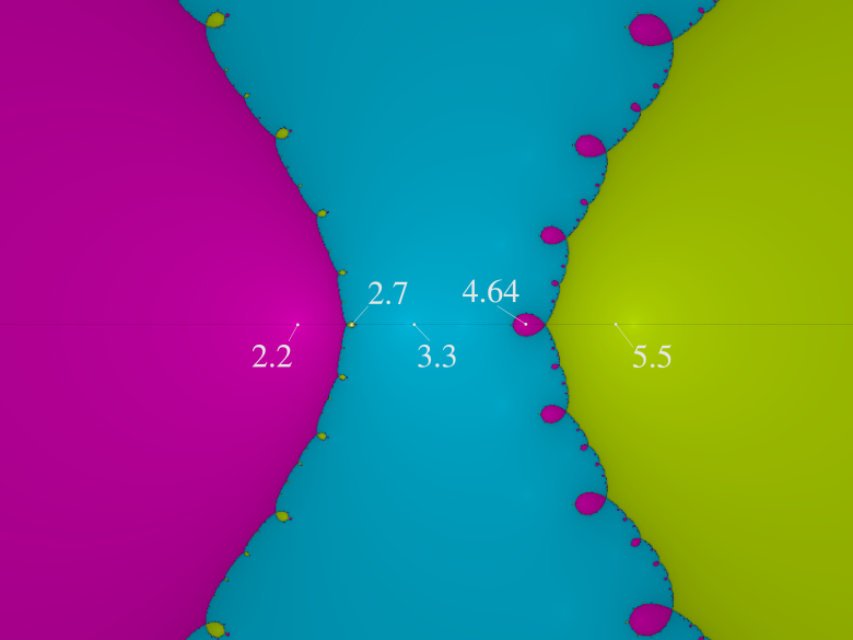
$Julia set for the function (x-2.2)(x-3.3)(x-5.5). There is a large pink region on the left, a large yellow region on the right, and in between a large blue hourglass-shaped region. The boundary of yellow region is decorated with pink bobbles that protrude into the blue region, and similarly the boundary of the pink region is decorated with yellow bobbles. Further details are in the text below.$

The real axis is the horizontal hairline along the middle of the diagram. The three large regions are the main basins of attraction to the three roots (!!x=2.2, 3.3!!, and !!5.5!!) that lie within them.

But along the boundaries of each region are smaller intrusive bubbles where the iteration converges to a surprising value. A point moving from left to right along the real axis passes through the large pink !!2.2!! region, and then through a very small yellow bubble, corresponding to the values right around the local maximum near !!x=2.7!! where the process unexpectedly converges to the !!5.5!! root. Then things settle down for a while in the blue region, converging to the !!3.3!! root as one would expect, until the value gets close to the local minimum at !!4.64!! where there is a pink bubble because the iteration converges to the !!2.2!! root instead. Then as !!x!! increases from !!4.64!! to !!5.5!!, it leaves the pink bubble and enters the main basin of attraction to !!5.5!! and stays there.

If the picture were higher resolution, you would be able to see that the pink bubbles all have tiny yellow bubbles growing out of them (one is 4.39), and the tiny yellow bubbles have even tinier pink bubbles, and so on forever.

(This was generated by the Online Fractal Generator at usefuljs.net; the labels were added later by me. The labels’ positions are only approximate.)

[ Addendum: Regarding complex points and !!f : z\mapsto z^3-1!! I said “some nearish starting points are near an extremum”. But this isn't right; !!f!! has no extrema. It has an inflection point at !!z=0!! but this doesn't explain the instability along the lines !!\theta = \frac{2k+1}{3}\pi!!. So there's something going on here with the complex derivative that I don't understand yet. ]

[Other articles in category /math] permanent link

Fixed points and attractors, part 3

Last week I wrote about a super-lightweight variation on Newton's method, in which one takes this function: $$f_n : \frac ab \mapsto \frac{a+nb}{a+b}$$

or equivalently

$$f_n : x \mapsto \frac{x+n}{x+1}$$

Iterating !!f_n!! for a suitable initial value (say, !!1!!) converges to !!\sqrt n!!:

$$ \begin{array}{rr} x & f_3(x) \\ \hline 1.0 & 2.0 \\ 2.0 & 1.667 \\ 1.667 & 1.75 \\ 1.75 & 1.727 \\ 1.727 & 1.733 \\ 1.733 & 1.732 \\ 1.732 & 1.732 \end{array} $$

Later I remembered that a few months back I wrote a couple of articles about a more general method that includes this as a special case:

The general idea was:

Suppose we were to pick a function !!f!! that had !!\sqrt 2!! as a fixed point. Then !!\sqrt 2!! might be an attractor, in which case iterating !!f!! will get us increasingly accurate approximations to !!\sqrt 2!!.

We can see that !!\sqrt n!! is a fixed point of !!f_n!!:

$$ \begin{align} f_n(\sqrt n) & = \frac{\sqrt n + n}{\sqrt n + 1} \\ & = \frac{\sqrt n(1 + \sqrt n)}{1 + \sqrt n} \\ & = \sqrt n \end{align} $$

And in fact, it is an attracting fixed point, because if !!x = \sqrt n + \epsilon!! then

$$\begin{align} f_n(\sqrt n + \epsilon) & = \frac{\sqrt n + \epsilon + n}{\sqrt n + \epsilon + 1} \\ & = \frac{(\sqrt n + \sqrt n\epsilon + n) - (\sqrt n -1)\epsilon}{\sqrt n + \epsilon + 1} \\ & = \sqrt n - \frac{(\sqrt n -1)\epsilon}{\sqrt n + \epsilon + 1} \end{align}$$

Disregarding the !!\epsilon!! in the denominator we obtain $$f_n(\sqrt n + \epsilon) \approx \sqrt n - \frac{\sqrt n - 1}{\sqrt n + 1} \epsilon $$

The error term !!-\frac{\sqrt n - 1}{\sqrt n + 1} \epsilon!! is strictly smaller than the original error !!\epsilon!!, because !!0 < \frac{x-1}{x+1} < 1!! whenever !!x>1!!. This shows that the fixed point !!\sqrt n!! is attractive.

In the previous articles I considered several different simple functions that had fixed points at !!\sqrt n!!, but I didn't think to consider this unusally simple one. I said at the time:

I had meant to write about Möbius transformations, but that will have to wait until next week, I think.

but I never did get around to the Möbius transformations, and I have long since forgotten what I planned to say. !!f_n!! is an example of a Möbius transformation, and I wonder if my idea was to systematically find all the Möbius transformations that have !!\sqrt n!! as a fixed point, and see what they look like. It is probably possible to automate the analysis of whether the fixed point is attractive, and if not to apply one of the transformations from the previous article to make it attractive.

[Other articles in category /math] permanent link

Tue, 13 Oct 2020

Newton's Method but without calculus — or multiplication

Newton's method goes like this: We have a function !!f!! and we want to solve the equation !!f(x) = 0.!! We guess an approximate solution, !!g!!, and it doesn't have to be a very good guess.

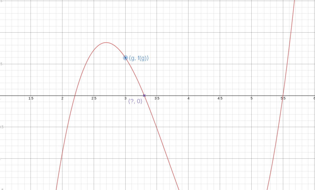
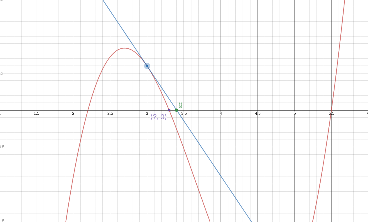
$The graph of a wiggly polynomial girve with roots between 2 and 2.5, between 3 and 3.5, and between 5 and 6. The middle root is labeled with a question mark. One point of the curve, not too different from the root, is marked in blue and labeled “⟨g,f(g)⟩”.$

Then we calculate the line !!T!! tangent to !!f!! through the point !!\langle g, f(g)\rangle!!. This line intersects the !!x!!-axis at some new point !!\langle \hat g, 0\rangle!!, and this new value, !!\hat g!!, is a better approximation to the value we're seeking.

$The same graph as before, but with a tangent to the curve drawn through the blue point. It intersects the x-axis quite close to the root. The intersection point is labeled “ĝ”.$

$In the left margin, a close-up detail of the same curve as before, this time showing the tangent line at ⟨ĝ,f(ĝ)⟩. The diagram is a close-up because the line intersects the x-axis extremely close to the actual root.$

Analytically, we have:

$$\hat g = g - \frac{f(g)}{f'(g)}$$

where !!f'(g)!! is the derivative of !!f!! at !!g!!.

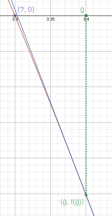
We can repeat the process if we like, getting better and better approximations to the solution. (See detail at left; click to enlarge. Again, the blue line is the tangent, this time at !!\langle \hat g, f(\hat g)\rangle!!. As you can see, it intersects the axis very close to the actual solution.)

In general, this requires calculus or something like it, but in any particular case you can avoid the calculus. Suppose we would like to find the square root of 2. This amounts to solving the equation $$x^2-2 = 0.$$ The function !!f!! here is !!x^2-2!!, and !!f'!! is !!2x!!. Once we know (or guess) !!f'!!, no further calculus is needed. The method then becomes: Guess !!g!!, then calculate $$\hat g = g - \frac{g^2-2}{2g}.$$ For example, if our initial guess is !!g = 1.5!!, then the formula above tells us that a better guess is !!\hat g = 1.5 - \frac{2.25 - 2}{3} = 1.4166\ldots!!, and repeating the process with !!\hat g!! produces !!1.41421\mathbf{5686}!!, which is very close to the correct result !!1.41421\mathbf{3562}!!. If we want the square root of a different number !!n!! we just substitute it for the !!2!! in the numerator.

This method for extracting square roots works well and requires no calculus. It's called the Babylonian method and while there's no evidence that it was actually known to the Babylonians, it is quite ancient; it was first recorded by Hero of Alexandria about 2000 years ago.

How might this have been discovered if you didn't have calculus? It's actually quite easy. Here's a picture of the number line. Zero is at one end, !!n!! is at the other, and somewhere in between is !!\sqrt n!!, which we want to find.

$A line with the left enpoint marked “0”, the right endpoint marked “n”, and a point in between marked “square root of n”.$

Also somewhere in between is our guess !!g!!. Say we guessed too low, so !!0 \lt g < \sqrt n!!. Now consider !!\frac ng!!. Since !!g!! is too small to be !!\sqrt n!! exactly, !!\frac ng!! must be too large. (If !!g!! and !!\frac ng!! were both smaller than !!\sqrt n!!, then their product would be smaller than !!n!!, and it isn't.)

$The previous illustration, with green points marked “g” and “\frac{n}{g}”. The first of these it to the left of the square root of n, the second to its right.$

Similarly, if the guess !!g!! is too large, so that !!\sqrt n < g!!, then !!\frac ng!! must be less than !!\sqrt n!!. The important point is that !!\sqrt n!! is between !!g!! and !!\frac ng!!. We have narrowed down the interval in which !!\sqrt n!! lies, just by guessing.

Since !!\sqrt n!! lies in the interval between !!g!! and !!\frac ng!! our next guess should be somewhere in this smaller interval. The most obvious thing we can do is to pick the point halfway in the middle of !!g!! and !!\frac ng!!, So if we guess the average, $$\frac12\left(g + \frac ng\right),$$ this will probably be much closer to !!\sqrt n!! than !!g!! was:

$The previous illustration, but the point exactly midway between g and \frac{n}{g} is marked in blue. It is quote close to the point marked “square root of n”.$

This average is exactly what Newton's method would have calculated, because $$\frac12\left(g + \frac ng\right) = g - \frac{g^2-n}{2g}.$$

But we were able to arrive at the same computation with no calculus at all — which is why this method could have been, and was, discovered 1700 years before Newton's method itself.

If we're dealing with rational numbers then we might write !!g=\frac ab!!, and then instead of replacing our guess !!g!! with a better guess !!\frac12\left(g + \frac ng\right)!!, we could think of it as replacing our guess !!\frac ab!! with a better guess !!\frac12\left(\frac ab + \frac n{\frac ab}\right)!!. This simplifies to

$$\frac ab \Rightarrow \frac{a^2 + nb^2}{2ab}$$

so that for example, if we are calculating !!\sqrt 2!!, and we start with the guess !!g=\frac32!!, the next guess is $$\frac{3^2 + 2\cdot2^2}{2\cdot3\cdot 2} = \frac{17}{12} = 1.4166\ldots$$ as we saw before. The approximation after that is !!\frac{289+288}{2\cdot17\cdot12} = \frac{577}{408} = 1.41421568\ldots!!. Used this way, the method requires only integer calculations, and converges very quickly.

But the numerators and denominators increase rapidly, which is good in one sense (it means you get to the accurate approximations quickly) but can also be troublesome because the numbers get big and also because you have to multiply, and multiplication is hard.

But remember how we figured out to do this calculation in the first place: all we're really trying to do is find a number in between !!g!! and !!\frac ng!!. We did that the first way that came to mind, by averaging. But perhaps there's a simpler operation that we could use instead, something even easier to compute?

Indeed there is! We can calculate the mediant. The mediant of !!\frac ab!! and !!\frac cd!! is simply $$\frac{a+c}{b+d}$$ and it is very easy to show that it lies between !!\frac ab!! and !!\frac cd!!, as we want.

So instead of the relatively complicated $$\frac ab \Rightarrow \frac{a^2 + nb^2}{2ab}$$ operation, we can try the very simple and quick $$\frac ab \Rightarrow \operatorname{mediant}\left(\frac ab, \frac{nb}{a}\right) = \frac{a+nb}{b+a}$$ operation.

Taking !!n=2!! as before, and starting with !!\frac 32!!, this produces:

$$ \frac 32 \Rightarrow\frac{ 7 }{ 5 } \Rightarrow\frac{ 17 }{ 12 } \Rightarrow\frac{ 41 }{ 29 } \Rightarrow\frac{ 99 }{ 70 } \Rightarrow\frac{ 239 }{ 169 } \Rightarrow\frac{ 577 }{ 408 } \Rightarrow\cdots$$

which you may recognize as the convergents of !!\sqrt2!!. These are actually the rational approximations of !!\sqrt 2!! that are optimally accurate relative to the sizes of their denominators. Notice that !!\frac{17}{12}!! and !!\frac{577}{408}!! are in there as they were before, although it takes longer to get to them.

I think it's cool that you can view it as a highly-simplified version of Newton's method.

[ Addendum: An earlier version of the last paragraph claimed:

None of this is a big surprise, because it's well-known that you can get the convergents of !!\sqrt n!! by applying the transformation !!\frac ab\Rightarrow \frac{a+nb}{a+b}!!, starting with !!\frac11!!.

Simon Tatham pointed out that this was mistaken. It's true when !!n=2!!, but not in general. The sequence of fractions that you get does indeed converge to !!\sqrt n!!, but it's not usually the convergents, or even in lowest terms. When !!n=3!!, for example, the numerators and denominators are all even. ]

[ Addendum: Newton's method as I described it, with the crucial !!g → g - \frac{f(g)}{f'(g)}!! transformation, was actually invented in 1740 by Thomas Simpson. Both Isaac Newton and Thomas Raphson had earlier described only special cases, as had several Asian mathematicians, including Seki Kōwa. ]

[ Previous discussion of convergents: Archimedes and the square root of 3; 60-degree angles on a lattice. A different variation on the Babylonian method. ]

[ Note to self: Take a look at what the AM-GM inequality has to say about the behavior of !!\hat g!!. ]

[ Addendum 20201018: A while back I discussed the general method of picking a function !!f!! that has !!\sqrt 2!! as a fixed point, and iterating !!f!!. This is yet another example of such a function. ]

[Other articles in category /math] permanent link