Mark Dominus (陶敏修)
mjd@pobox.com

Archive:
| 2026: | JFM |
| 2025: | JFMAMJ |
| JASOND | |
| 2024: | JFMAMJ |
| JASOND | |
| 2023: | JFMAMJ |
| JASOND | |
| 2022: | JFMAMJ |
| JASOND | |
| 2021: | JFMAMJ |
| JASOND | |
| 2020: | JFMAMJ |
| JASOND | |
| 2019: | JFMAMJ |
| JASOND | |
| 2018: | JFMAMJ |
| JASOND | |
| 2017: | JFMAMJ |
| JASOND | |
| 2016: | JFMAMJ |
| JASOND | |
| 2015: | JFMAMJ |
| JASOND | |
| 2014: | JFMAMJ |
| JASOND | |
| 2013: | JFMAMJ |
| JASOND | |
| 2012: | JFMAMJ |
| JASOND | |
| 2011: | JFMAMJ |
| JASOND | |
| 2010: | JFMAMJ |
| JASOND | |
| 2009: | JFMAMJ |
| JASOND | |
| 2008: | JFMAMJ |
| JASOND | |
| 2007: | JFMAMJ |
| JASOND | |
| 2006: | JFMAMJ |
| JASOND | |
| 2005: | OND |
In this section:
Subtopics:
| Mathematics | 246 |
| Programming | 100 |
| Language | 95 |
| Miscellaneous | 75 |
| Book | 50 |
| Tech | 49 |
| Etymology | 36 |
| Haskell | 33 |
| Oops | 30 |
| Unix | 27 |
| Cosmic Call | 25 |
| Math SE | 25 |
| Law | 23 |
| Physics | 21 |
| Perl | 17 |
| Biology | 16 |
| Brain | 15 |
| Calendar | 15 |
| Food | 15 |


Comments disabled
Mon, 22 Jan 2007
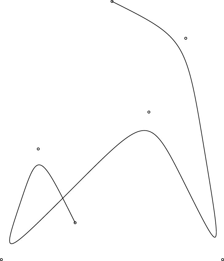
Linogram circular problems
The problems are not related to geometric circles; the are logically
circular.
 In the course of preparing my sample curve diagrams, one of which is
shown at right, I ran into several related bugs in the way that arrays
were being handled. What I really wanted to do was to define a
labeled_curve object, something like this:
In the course of preparing my sample curve diagrams, one of which is
shown at right, I ran into several related bugs in the way that arrays
were being handled. What I really wanted to do was to define a
labeled_curve object, something like this:
        define labeled_curve extends curve {
          spot s[N];
          constraints { s[i] = control[i]; }
        }
That is, it is just like an ordinary curve, except that it also has a
"spot" at each control point. A "spot" is a graphic element that
marks the control point, probably with a small circle or something of
the sort:
        define spot extends point {
           circle circ(r=0.05);
           constraints {
             circ.c.x = x;  circ.c.y = y;
           }
        }
A spot is like a point, and so it has an x
and a y coordinate. But it also has a circle, circ,
which is centered at this location. (circ.c is the center of
the circle.)When I first tried this, it didn't work because linogram didn't understand that a labeled_curve with N = 4 control points would also have four instances of circ, four of circ.c, four of circ.c.x, and so on. It did understand that the labeled curve would have four instances of s, but the multiplicity wasn't being propagated to the subobjects of s.
I fixed this up in pretty short order.
But the same bug persisted for circ.r, and this is not so easy to fix. The difference is that while circ.c is a full subobject, subject to equation solving, and expected to be unknown, circ.r is a parameter, which much be specified in advance.
N, the number of spots and control points, is another such parameter. So there's a first pass through the object hierarchy to collect the parameters, and then a later pass figures out the subobjects. You can't figure out the subobjects without the parameters, because until you know the value of parameters like N, you don't know how many subobjects there are in arrays like s[N].
For subobjects like S[N].circ.c.x, there is no issue. The program gathers up the parameters, including N, and then figures out the subobjects, including S[0].circ.c.x and so on. But S[0].circ.r, is a parameter, and I can't say that its value will be postponed until after the values of the parameters are collected. I need to know the values of the parameters before I can figure out what the parameters are.
This is not a show-stopper. I can think of at least three ways forward. For example, the program could do a separate pass for param index parameters, resolving those first. Or I could do a more sophisticated dependency analysis on the parameter values; a lot of the code for this is already around, to handle things like param number a = b*2, b=4, c=a+b+3, d=c*5+b. But I need to mull over the right way to proceed.
Consider this oddity in the meantime:
  define snark {
    param number p = 3;
  }
  define boojum {
    param number N = s[2].p;
    snark s[N];
  }
Here the program needs to know the value of N in order to
decide how many snarks are in a boojum. But the number N itself is
determined by examining the p parameter in snark 2, which
itself will not exist if N is less than 3. Should this sort of
nonsense be allowed? I'm not sure yet.When you invent a new kind of program, there is an interesting tradeoff between what you want to allow, what you actually do allow, and what you know how to implement. I definitely want to allow the labeled_curve thing. But I'm quite willing to let the snark-boojum example turn into some sort of run-time failure.
[Other articles in category /linogram] permanent link
Sun, 21 Jan 2007
Recent Linogram development update
Lately most of my spare time (and some not-spare time) has been going
to linogram. I've been posting updates pretty regularly at
the main linogram page. But I don't know if
anyone ever looks at that page. That got me thinking that it was not
convenient to use, even for people who are interested in
linogram, and that maybe I should have an RSS/Atom feed for
that page so that people who are interested do not have to keep
checking back.
Then I said "duh", because I already have a syndication feed for this page, so why not just post the stuff here?
So that is what I will do. I am about to copy a bunch of stuff from that page to this one, backdating it to match when I posted it.
The new items are: [1] [2] [3] [4] [5].
People who only want to hear about linogram, and not about
anything else, can subscribe to
 this RSS feed
or
this Atom feed.
this RSS feed
or
this Atom feed.
[Other articles in category /linogram] permanent link
Sat, 20 Jan 2007
Another Linogram success story
I've been saying for a while that a well-designed system surprises
even the designer with its power and expressiveness. Every time
linogram surprises me, I feel a flush of satisfaction because
this is evidence that I designed it well. I'm beginning to think that
linogram may be the best single piece of design I've
ever done.
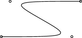
Here was today's surprise. For a long time, my demo diagram has been a rough rendering of one of the figures from Higher-Order Perl:

I wanted component k in the middle of the diagram to be a curved line, but since I didn't have curved lines yet, I used two straight lines instead, as shown below:
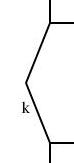
        define bentline {
          line upper, lower;
          param number depth = 0.2;
          point start, end, center;
          constraints {
            center = upper.end = lower.start;
            start = upper.start;  end = lower.end;
            start.x = end.x = center.x + depth;
            center.y = (start.y + end.y)/2;
          }
        }

        ...

        bentline k;
        label klbl(text="k") = k.upper.center - (0.1, 0);
        ...
        constraints {
          ...
          k.start = plus.sw; k.end = times.nw;
          ...
        }
So I had defined a thing called a bentline, which is a line
with a slight angle in it. Or more precisely, it's two
approximately-vertical lines joined end-to-end. It has three
important reference points: start, which is the top point,
end, the bottom point, which is directly under the top
point, and center, halfway in between, but displaced
leftward by depth. I now needed to replace this with a curved line. This meant removing all the references to start, end, upper and so forth, since curves don't have any of those things. A significant rewrite, in other words.
But then I had a happy thought. I added the following definition to the file:
        require "curve";
        define bentline_curved extends bentline {
          curve c(N=3);
          constraints {
            c.control[0] = start;
            c.control[1] = center;
            c.control[2] = end;
          }
          draw { c; }
        }
A bentline_curved is now the same as a bentline, but
with an extra curved line, called c, which has three control
points, defined to be identical with start, center,
and end. These three points inherit all the same constraints
as before, and so are constrained in the same way and positioned in
the same way. But instead of drawing the two lines, the
bentline_curved draws only the curve. I then replaced:
bentline k;
with:
bentline_curved k;
and recompiled the diagram. The result is below:
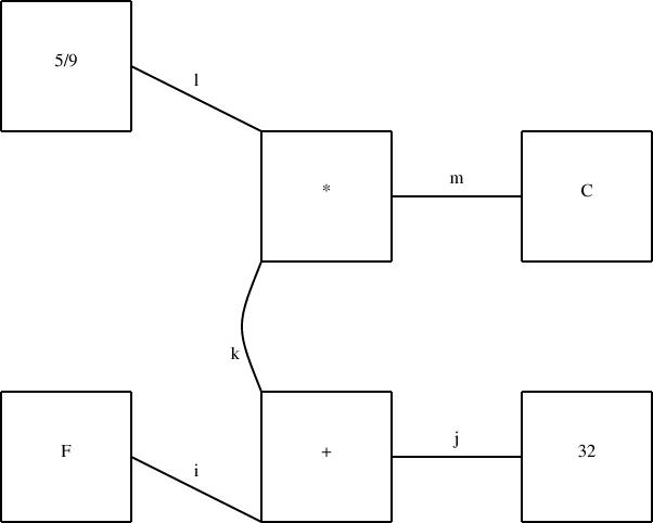
| | 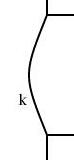
|
I didn't foresee this when I designed the linogram language. Sometimes when you try a new kind of program for the first time, you keep getting unpleasant surprises. You find things you realize you didn't think through, or that have unexpected consequences, or features that turn out not to be as powerful as you need, or that mesh badly with other features. Then you have to go back and revisit your design, fix problems, try to patch up mismatches, and so forth. In contrast, the appearance of the sort of pleasant surprise like the one in this article is exactly the opposite sort of situation, and makes me really happy.
[Other articles in category /linogram] permanent link
Linogram development: 20070120 Update
The array feature is working, pending some bug fixes. I have not yet
found all the bugs, I think. But the feature has definitely moved
from the does-not-work-at-all phase into the mostly-works phase. That
is, I am spending most of my time tracking down bugs, rather than
writing large amount of code. The test suite is expanding rapidly.
The regular polygons are working pretty well, and the curves are working pretty well. Here are some simple examples:
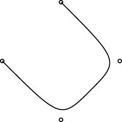
| 
|
One interesting design problem turned up that I had not foreseen. I had planned for the curve object to be specified by 2 or more control points. (The control points are marked by little circles in the demo pictures above.) The first and last controlpoints would be endpoints, and the curve would start at point 0, then head toward point 1, veer off toward point 2, then veer off toward point 3, etc., until it finally ended at point N. You can see this in the pictures.
This is like the behavior of pic, which has good-looking curves. You don't want to require that the curve pass through all the control points, because that does not give it enough freedom to be curvy. And this behavior is easy to get just by using a degree-N Bézier curve, which was what I planned to do.
However, PostScript surprised me. I had thought that it had degree-N Bézier curves, but it does not. It has only degree-3 ("cubic") Bézier curves. So then I was left with the puzzle of how to use PostScript's Bézier curves to get what I wanted. Or should I just change the definition of curve in linogram to be more like what PostScript wanted? Well, I didn't want to do that, because linogram is supposed to be generic, not a front-end to PostScript. Or, at least, not a front-end only to PostScript.
I did figure out a compromise. The curves generated by the PostScript drawer are made of PostScript's piecewise-cubic curves, but, as you can see from the demo pictures, they still have the behavior I want. The four control points in the small demos above actually turn into two PostScript cubic Bézier curves, with a total of seven control points. If you give linogram the points A, B, C, and D, the PostScript engine draws two cubic Bézier curves, with control points {A, B, B, (B + C)/2} and {(B + C)/2, C, C, D}, respectively. Maybe I'll write a blog article about why I chose to do it this way.
One drawback of this approach is that the curves turn rather sharply near the control points. I may tinker with the formula later to smooth out the curves a bit, but I think for now this part is good enough for beta testing.
[Other articles in category /linogram] permanent link
Wed, 17 Jan 2007
Linogram development: 20070117 Update
The array feature is almost complete, perhaps entirely complete.
Fully nontrivial tests are passing. For example, here is test
polygon002 from the distribution:
        require "polygon";

        polygon t1(N=3), t2(N=3);

        constraints {
          t1.v[0] = (0, 0);
          t1.v[1] = (1, 1);
          t1.v[2] = (2, 3);
          t2.v[i] = t1.v[i-1];
        }
This defines two polygons, t1 and
t2, each with three sides. The three vertices of
t1 are specified explicitly. Triangle
t2 is the same, but with the vertices numbered
differently: t2.v0 =
t1.v2,
t2.v1 =
t1.v0, and
t2.v2 =
t1.v1. Each of the triangles also
has three edges, defined implicitly by the definition in
polygon.lino:
        require "point";
        require "line";

        define polygon {
          param index N;
          point v[N];
          line e[N];
          constraints {
            e[i].start = v[i];
            e[i].end = v[i+1];
          }
        }
All together, there are 38 values here: 2 coordinates for each of
three vertices of each of the two triangles makes 12; 2 coordinates
for each of two endpoints of each of three edges of each of the two
triangles is another 24, and the two N values themselves
makes a total of 12 + 24 + 2 = 38.All of the equations are rather trivial. All the difficulty is in generating the equations in the first place. The program must recognize that the variable i in the polygon definition is a dummy iterator variable, and that it is associatated with the parameter N in the polygon definition. It must propagate the specification of N to the right place, and then iterate the equations appropriately, producing something like:
e0.end = v0+1Then it must fold the constants in the subscripts and apply the appropriate overflow semantics—in this case, 2+1=0.
e1.end = v1+1
e2.end = v2+1
Open figures still don't work properly. I don't think this will take too long to fix.
The code is very messy. For example, all the Type classes are in a file whose name is not Type.pm but Chunk.pm. I plan to have a round of cleanup and consolidation after the 2.0 release, which I hope will be soon.
[Other articles in category /linogram] permanent link
Wed, 27 Dec 2006
Linogram development: 20061227 Update
Defective constraints (see yesterday's article)
are now handled. So the example from yesterday's
article has now improved to:
        define regular_polygon[N] closed {
          param number radius, rotation=0;
          point vertex[N], center;
          line  edge[N];
          constraints {
            vertex[i] = center + radius * cis(rotation + 360*i/N);
            edge[i].start = vertex[i];
            edge[i].end   = vertex[i+1];
          }
        }
[Other articles in category /linogram] permanent link
Tue, 26 Dec 2006
Linogram development: 20061226 Update
I have made significant progress on the "arrays" feature. I
recognized that it was actually three features; I have two of them
implemented now. Taking the example from further down the page:
        define regular_polygon[N] closed {
          param number radius, rotation=0;
          point vertex[N], center;
          line  edge[N];
          constraints {
            vertex[i] = center + radius * cis(rotation + 360*i/N);
            edge[i].start = vertex[i];
            edge[i].end   =  vertex[i+1];
          }
        }
The stuff in green is working just right; the stuff in red is not.The following example works just fine:
        number p[3];
        number q[3];
        constraints {
          p[i] = q[i];
          q[i] = i*2;
        }
What's still missing? Well, if you write
        number p[3];
        number q[3];
        constraints {
          p[i] = q[i+1];
        }
This should imply three constraints on elements of p and
q:
p0 = q1
p1 = q2
p2 = q3
The third of these is defective, because there is no q3. If the figure is "closed" (which is the default) the subscripts should wrap around, turning the defective constraint into p2 = q0 instead. If the figure is declared "open", the defective constraint should simply be discarded.
The syntax for parameterized definitions (define regular_polygon[N] { ... }) is still a bit up in the air; I am now leaning toward a syntax that looks more like define regular_polygon { param index N; ... } instead.
The current work on the "arrays" feature is in the CVS repository on the branch arrays; get the version tagged tests-pass to get the most recent working version. Most of the interesting work has been on the files lib/Chunk.pm and lib/Expression.pm.
[Other articles in category /linogram] permanent link
Thu, 23 Nov 2006
Linogram: The EaS as a component
In an earlier article, I
discussed the definition of an Etch-a-Sketch picture as a component in the linogram
drawing system. I then digressed for a day to rant
about the differences between specification-based and WYSIWYG
systems. I now return to the main topic.
Having defined the EAS component, I can use it in several diagrams. The typical diagram looks like this:
        require "eas";

        number WIDTH = 2;

        EAS the_eas(w = WIDTH);

        gear3 gears(width=WIDTH, r1=1/4, r3=1/12);

        constraints {
            the_eas.left = gears.g1.c;
            the_eas.right = gears.g3.c;
        }
The eas.lino file defines the EAS component and also
the gear3 component, which describes what the three gears
should look like. The diagram itself just chooses a global width and
communicates it to the EAS component and the gear3
component. It also communicates two of the three selected gear sizes
to the gear3, which generates the three gears and their
axles. Finally, the specification constrains the left
reference point of the Etch-a-Sketch to lie at the center of gear 1, and the
right reference point to lie at the center of gear 3.This sort of thing was exactly what I was hoping for when I started designing linogram. I wanted it to be easy to define a new component type, like EAS or gear3, and to use it as if it were a built-in type. (Indeed, as noted before, even linogram's "built-in" types are not actually built in! Everything from point on up is defined by a .lino file just like the one above, and if the user wants to redefine point or line, they are free to do so.)
(It may not be clear redefining point or line is actually a useful thing to do. But it could be. Consider, for example, what would happen if you were to change the definition of point to contain a z coordinate, in addition to the x and y coordinates it normally has. The line and box definitions would inherit this change, and become three-dimensional objects. If provided with a suitably enhanced rendering component, linogram would then become a three-dimensional diagram-drawing program. Eventually I will add this enhancement to linogram.)
I am a long-time user of the AT&T Unix tool pic, which wants to allow you to define and use compound objects in this way, but gets it badly wrong, so that it's painful and impractical. Every time I suffered through pic's ineptitude, I would think about how it might be done properly. I think linogram gets it right; pic was a major inspiration.
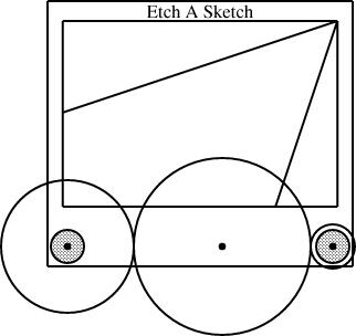
Slanty lines
Partway through drawing the Etch-a-Sketch diagrams, I had a happy idea. Since I was describing Etch-a-Sketch configurations that would draw lines with various slopes, why not include examples?
line L(slope=..., start=..., ...);
In general, though, this is too hard to handle. The resulting equations are quadratic, or worse, trigonometric, and linogram does not know how to solve those kinds of equations.
But if the slope is required to be constant, then the quadratic equations become linear, and there is no problem. And in this case, I only needed constant slopes. Once I realized this, it was easy to define a constant-slope line type:
        require "line";

        define sline extends line {
          param number slope;
          constraints {
            end.y - start.y = slope * (end.x - start.x);
          }
        }
An sline is just like a line, but it has an
additional parameter, slope (which must be constant, and
specified at compile time, not inferred from other values) and one
extra constraint that uses it. Normally, all four of start.x,
end.x, start.y, and end.y are independent.
The constraint removes some of the independence, so that any three,
plus the slope, are sufficient to determine the fourth.The diagram above was generated from this specification:
        require "eas";
        require "sline";

        number WIDTH = 2;

        EAS the_eas(w = WIDTH);

        gear3 gears(width=WIDTH, r1=1/4, r3=1/12);
        sline L1(slope=1/3, start=the_eas.screen.ne);
        sline L2(slope=3, start=the_eas.screen.ne);

        constraints {
            the_eas.left = gears.g1.c;
            the_eas.right = gears.g3.c;
            L1.end.x = the_eas.screen.w.x;
            L2.end.y = the_eas.screen.s.y;
        }
The additions here are the sline items, named L1 and L2. Both lines start at the northeast corner of the screen. Line L1 has slope 1/3, and its other endpoint is constrained to lie somewhere on the west edge of the screen. The y-coordinate of that endpoint is not specified, but is implicitly determined by the other constraints. To locate it, linogram must solve some linear equations. The complete set of constraints no the line is:
| L1.start.x = the_eas.screen.ne.x |
| L1.start.y = the_eas.screen.ne.y |
| L1.end.x = the_eas.screen.w.x |
| L1.end.y - L1.start.y = L1.slope × (L1.end.x - L1.start.x); |
| L1.end.y - L1.start.y = 1/3 × (L1.end.x - L1.start.x); |
The other line, L2, with slope 3, is handled similarly; its endpoint is constrained to lie somewhere on the south side of the screen.
Surprise features
When I first planned linogram, I was hardly thinking of slopes at all, except to dismiss them as being intractable, along with a bunch of other things like angles and lengths. But it turned out that they are a little bit tractable, enough that linogram can get a bit of a handle on them, thanks to the param feature that allows them to be excluded from the linear equation solving.One of the signs that you have designed a system well is that it comes out to be more powerful than you expected when you designed it, and lends itself to unexpected uses. The slines are an example of that. When it occurred to me to try doing them, my first thought was "but that won't work, will it?" But it does work.
Here's another technique I hadn't specifically planned for, that is already be supported by linogram. Suppose Fred Flooney wants to use the eas library, but doesn't like the names of the reference points in the EAS component. Fred is quite free to define his own replacement, with whatever names for whatever reference points he likes
        require "eas";

        define freds_EAS {
          EAS it;
          point middle = it.screen.c;
          point bernard = (it.body.e + 2*it.body.se)/3;
          line diag(start=it.body.nw, end=it.body.se);
          draw { it; }
        }
The freds_EAS component is essentially the same as the
EAS component defined by eas.lino. It contains a
single Etch-a-Sketch, called it, and a few extra items that Fred is
interested in. If E is a freds_EAS, then
E.middle refers to the point at the center of E's
screen; E.bernard is a point two-thirds of the way between
the middle and the bottom corner of its outer edge, and
E.diag is an invisible line running diagonally across the
entire body, equipped with the usual E.diag.start,
E.diag.center, and the like. All the standard items are
still available, as E.it.vknob,
E.it.screen.left.center, and so on.
The draw section tells linogram that only the component named it—that is, the Etch-a-Sketch itself—should be drawn; this suppresses the diag line. which would otherwise have been rendered also.
If Fred inherits some other diagram or component that includes an Etch-a-Sketch, he can still use his own aliases to refer to the parts of the Etch-a-Sketch, without modifying the diagram he inherited. For example, suppose Fred gets handed my specification for the diagram above, and wants to augment it or incorporate it in a larger diagram. The diagram above is defined by a file called "eas4-3-12.lino", which in turn requires EAS.lino. Fred does not need to modify eas4-3-12.lino; he can do:
        require "eas4-3-12.lino";
        require "freds_eas";

        freds_EAS freds_eas(it = the_eas);

        constraints {
          freds_eas.middle = ...;
          freds_eas.bernard = ...;
        }
        ...
Fred has created one of his extended Etch-a-Sketch components, and identified
the Etch-a-Sketch part of it with the_eas, which is the Etch-a-Sketch part of my
original diagram. Fred can then apply constraints to the
middle and bernard sub-parts of his
freds_eas, and these constraints will be propagated to the
corresponding parts the the_eas in my original diagram. Fred
can now specify relations in terms of his own peronal middle
and bernard items, and they will automatically be related to
the appropriate parts of my diagram, even though I have never heard of
Fred and have no idea what bernard is supposed to represent.Why Fred wants these names for these components, I don't know; it's just a contrived example. But the important point is that if he does want them, he can have them, with no trouble.
What next?
There are still a few things missing from linogram. The last major missing feature is arrays. The gear3 construction I used above is clumsy. It contains a series of constraints that look like:
  g1.e = g2.w;
  g2.e = g3.w;
The same file also has an analogous gear2 definition, for diagrams with only two gears. Having both gear2 and gear3, almost the same, is silly and wasteful. What I really want is to be able to write:
  define gears[n] open {
    gear[n] g;
    constraints {
      g[i].e = g[i+1].w;
    }
  }
and this would automatically imply components like gear2 and
gear3, with 2 and 3 gears, but denoted gear[2] and gear[3],
respectively; it would also imply gear[17] and
gear[253] with the analogous constraints.For gear[3], two constraints are generated: g[0].e = g[1].w, and g[1].e = g[2].w. Normally, arrays are cyclic, and a third constraint, g[2].e = g[0].w, would be generated as well. The open keyword suppresses this additional constraint.
This feature is under development now. I originally planned it to support splines, which can have any number of control points. But once again, I found that the array feature was going to be useful for many other purposes.
When the array feature is finished, the next step will be to create a spline type: spline[4] will be a spline with 4 control points; spline[7] will be a spline with 7 control points, and so on. PostScript will take care of drawing the splines for me, so that will be easy. I will also define a regular polygon type at that time:
        define polygon[n] closed {
          param number rotation = 0;
          number radius;
          point v[n], center;
          line  e[n];
          constraints {
            v[i] = center + radius * cis(rotation + i * 360/n);
            e[i].start = v[i];
            e[i].end   = v[i+1];
          }
        }
polygon[3] will then be a rightward-pointing equilateral
triangle; constraining any two of its vertices will determine the
position of the third, which will be positioned automatically. Note
the closed keyword, which tells linogram to include the constraint
e[2].end =
v[0], which would have been omitted had open been
used instead. More complete information about linogram is available in Chapter 9 of Higher-Order Perl; complete source code is available from the linogram web site.

[Other articles in category /linogram] permanent link
Wed, 22 Nov 2006
Linogram: Declarative drawing
As we saw in yesterday's
article, The definition of the EAS component is twenty
lines of strange, mostly mathematical notation. I could have drawn
the Etch-a-Sketch in a WYSIWYG diagram-drawing system like xfig. It might have
been less trouble. Many people will prefer this. Why invent linogram?
Some of the arguments should be familiar to you. The world is full of operating systems with GUIs. Why use the Unix command line? The world is full of WYSIWYG word processors. Why use TeX?
Text descriptions of processes can be automatically generated, copied, and automatically modified. Common parts can be abstracted out. This is a powerful paradigm.
Collectively, the diagrams contained 19 "gears". Partway through, I decided that the black dot that represented the gear axle was too small, and made it bigger. Had I been using a WYSIWYG system, I would have had the pleasure of editing 19 black dots in 10 separate files. Then, if I didn't like the result, I would have had the pleasure of putting them back the way they were. With linogram, all that was required was to change the 0.02 to an 0.05 in eas.lino:
        define axle {
          param number r = 0.05;
          circle a(fill=1, r=r);
        }
The Etch-a-Sketch article contained seven similar diagrams with slight differences. Each one contained a require "eas"; directive to obtain the same definition of the EAS component. Partway through the process, I decided to alter the aspect ratio of the Etch-a-Sketch body. Had I been drawing these with a WYSIWYG system, that would have meant editing each of the seven diagrams in the same way. With linogram, it meant making a single trivial change to eas.lino.
A linogram diagram has a structure: it is made up of component parts with well-defined relationships. A line in a WYSIWYG diagram might be 4.6 inches long. A line in a linogram diagram might also be 4.6 inches long, but that is probably not all there is to it. The south edge of the body box in my diagrams is 4.6 inches long, but only because it has been inferred (from other relationships) to be 1.15 w, and because w was specified to be 4 inches. Change w, and everything else changes automatically to match. Each part moves appropriately, to maintain the specified relationships. The distance from the knob centers to the edge remains 3/40 of the distance between the knobs. The screen remains 70% as tall as the body. A WYSIWYG system might be able to scale everything down by 50%, but all it can do is to scale down everything by 50%; it doesn't know enough about the relationships between the elements to do any better. What will happen if I reduce the width but not the height by 50%? The gears are circles; will the WYSIWYG system keep them as circles? Will they shrink appropriately? Will their widths be adjusted to fit between the two knobs? Maybe, or maybe not. In linogram, the required relationships are all explicit. For example, I specified the size of the black axle dots in absolute numbers, so they do not grow or shrink when the rest of the diagram is scaled.
Finally, because the diagrams are mathematically specified, I can leave the definitions of some of the components implicit in the mathematics, and let linogram figure them out for me. For example, consider this diagram:

gear3 gears(width=WIDTH, r1=1/4, r3=1/12);
I specified r1, the radius of the left gear, and r3, the radius of the right gear. Where is the middle gear? It's implicit in the definition of the gear3 type. The definition knows that the three gears must all touch, so it calculates the radius of the middle gear accordingly:
define gear3 {
  ...
  number r2 = (1 - r1 - r3) / 2;
  ...
}
linogram gives me the option of omitting r2 and having it be calculated for me from this formula, or of specifying r2 anyway, in which case linogram will check it against this formula and raise an error if the values don't match.
Tomorrow: The Etch-a-Sketch as a component.
More complete information about linogram is available in Chapter 9 of Higher-Order Perl; complete source code is available from the linogram web site.
[Other articles in category /linogram] permanent link
Tue, 21 Nov 2006
Linogram: The EaS component
In yesterday's article I
talked about the basic facilities provided by linogram. What about the
Etch-a-Sketch diagrams?
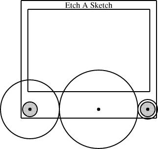
The core of these diagrams was a specification I wrote for an Etch-a-Sketch itself, in a file called eas.lino. The specification is complicated, because an Etch-a-Sketch has many parts, but it is conceptually just like the definitions above: it defines a diagram component called an EAS that looks like an Etch-a-Sketch:
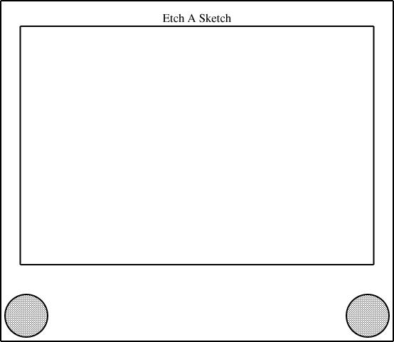
        define EAS {
          param number w;
          number knobrad = w * 1/16;
          circle hknob(r=knobrad, fill=0.25), vknob(r=knobrad, fill=0.25);
          point left = hknob.c, right = vknob.c;
          number margin = 3/40 * w;
          box body(sw = left + (-margin, -margin), se = right + (margin,  -margin),
                   ht = w * 1);
          box screen(wd = body.wd * 0.9,
                     n = body.n + (0, -margin),
                     ht = body.ht * 0.7);

          number nudge = body.ht * 0.025;
          label Brand(text="Etch A Sketch") = (body.n + screen.n)/2 + (0, -nudge);

          constraints { left + (w, 0) = right;
                        left.y = right.y = 0;
                        left.x = 0;
                      }
        }
I didn't, of course, write this all in one fell swoop. I built it up a bit at a time. Each time I changed the definition in the eas.lino file, the changes were inherited by all the files that contained require "eas".
The two main parts of the Etch-a-Sketch are the body (large outer rectangle) and screen (smaller inner rectangle), which are defined to be boxes:
        box body(...);
        box screen(...);
But most of the positions are ultimately referred to the centers of the two knobs. The knobs themselves are hknob and vknob, and their centers, hknob.c and vknob.c, are given the convenience names left and right:
point left = hknob.c, right = vknob.c;
Down in the constraints section is a crucial constraint:
left + (w, 0) = right;
This constrains the right point (and, by extension, vknob.c and the circle vknob of which it is the center, and, by further extension, anything else that depends on vknob) to lie exactly w units east and 0 units south of the left point. The number w ("width") is declared as a "param", and is special: it must be specified by the calling context, to tell the Etch-a-Sketch component how wide it is to be; if it is omitted, compilation of the diagram fails. By varying w, we can have linogram draw Etch-a-Sketch components in different sizes. The diagram above had w=4; this one has w=2:

number knobrad = w * 1/16;
So if you make w twice as big, the knobs get twice as big also.
The quantity margin is the amount of space between knobs and the edge of the body box, defined to be 3/40 of w:
number margin = 3/40 * w;
Since the margin is 0.075 w, and the knobs have size 0.0625 w, there is a bit of extra space between the knobs and the edge of the body. Had I wanted to state this explicitly, I could have defined margin = knobrad * 1.15 or something of the sort.
The southwest and southeast corners of the body box are defined as offsets from the left and right reference points, which are at the centers of the knobs:
          box body(sw = left + (-margin, -margin),
                   se = right + (margin, -margin),
                   ht = w * 1);
(The body(sw = ..., se = ..., ht = ...) notation is
equivalent to just including body.sw = ...; body.se =
...; body.ht = ... in the constraints section.)This implicitly specifies the width of the body box, since linogram can deduce it from the positions of the two bottom corners. The height of the body box is defined as being equal to w, making the height of the body equal to the distance between the to knobs. This is not realistic, since a real Etch-a-Sketch is not so nearly a square, but I liked the way it looked. Earlier drafts of the diagram had ht = w * 2/3, to make the Etch-a-Sketch more rectangular. Changing this one number causes linogram to adjust everything else in the entire diagram correspondingly; everything else moves around to match.
The smaller box, the screen, is defined in terms of the larger box, the body:
          box screen(wd = body.wd * 0.9,
                     n = body.n + (0, -margin),
                     ht = body.ht * 0.7);
It is 9/10 as wide as the body and 7/10 as tall. Its "north" point
(the middle of the top side) is due south of the north point of the
body, by a distance equal to margin, the distance between the
center of a knob and the bottom edge of the body. This is enough
information for linogram to figure out everything it needs to know about the
screen.The only other features are the label and the fill property of the knobs. A label is defined by linogram's standard library. It is like a point, but with an associated string:
        require "point";

        define label extends point {
                param string text;
                draw { &put_string; }
        }
Unlike an ordinary point, which is not drawn at all, a
label is drawn by placing the specified string at the
x and y coordinates of the point.
All the magic here is in the put_string() function, which is
responsible for generating the required PostScript output.
          number nudge = body.ht * 0.025;
          label Brand(text="Etch A Sketch") =
                (body.n + screen.n)/2 + (0, -nudge);
The text="..." supplies the text parameter, which is handed off directly to put_string(). The rest of the constraint says that the text should be positioned halfway between the north points of the body and the screen boxes, but nudged southwards a bit. The nudge value is a fudge factor that I put in because I haven't yet gotten the PostScript drawing component to position the text at the exact right location. Indeed, I'm not entirely sure about the best way to specify text positioning, so I left that part of the program to do later, when I have more experience with text.
The fill parameter of the knobs is handled similarly to the text parameter of a label: it's an opaque piece of information that is passed to the drawing component for handling:
circle hknob(r=knobrad, fill=0.25), vknob(r=knobrad, fill=0.25);
The PostScript drawing component then uses this when drawing the circles, eventually generating something like gsave 0.75 setgray fill grestore. The default value is 0, indicating white fill; here we use 0.25, which is light gray. (The PostScript drawing component turns this into 0.75, which is PostScript for light gray. PostScript has white=1 and black=0, but linogram has white=0 and black=1. I may reverse this before the final release, or make it a per-diagram configuration option.)
Tomorrow: Advantages of declarative drawing.
More complete information about linogram is available in Chapter 9 of Higher-Order Perl; complete source code is available from the linogram web site.
[Other articles in category /linogram] permanent link
Sun, 19 Nov 2006
A series of articles about Linogram
Every six months or so I do a little work on linogram, which for about
18 months now has been about one week of hard work short of version
1.0. Every time I try to use it, I am surprised by how pleased I am
with it, how easy I find it to use, and how flexible the (rather
spare) basic feature set is—all properties of a well-designed
system.
I was planning to write a short note about this, but, as always happens when I write about linogram, it turned into a very long note that included a tutorial about how linogram works, a rant about why it is a good idea, and a lot of technical examples. So I decided to break the 4,000-word article into smaller pieces, which I will serialize.
Most recently I used linogram to do schematic diagrams of an Etch-a-Sketch for some recent blog articles ([1] [2]). In case you have forgotten, here is an example:

Basic ideas of linogram
There are two basic concepts that provide the underpinnings of linogram. One is that most interesting features of a line drawing can be described by giving a series of linear equations that relate the positions of the components. For example, to say that line B starts at the same place that line A ends, one provides the two extremely simple linear equations:
        B.start.x = A.end.x;
        B.start.y = A.end.y;
which one can (and normally would) abbreviate to:
B.start = A.end;
The computer is very good at solving systems of linear equations, and can figure out all the things the equations imply. For example, consider two boxes, X and Y:
        X.ht = 2;     # height of box X
        Y.ht = 3;     # height of box Y
        X.s = Y.n;    # 's' is 'south'; 'n' is 'north'
From this, the program can deduce that the south edge of box Y
is 5 units south of the north edge of box X, even though
neither was mentioned explicitly.These simple examples are not very impressive, but please bear with me.
The other fundamental idea in linogram is the idea of elements of a diagram as components that can be composed into more complicated elements. The linogram libraries have a definition for a box, but it is not a primitive. In fact, linogram has one, and only one primitive type of element: the number. A point is composed of two numbers, called x and y, and is defined by the point.lino file in the library:
        define point {
          number x, y;
        }
A line can then be defined as an object that contains two points, the
start and end points:
        require "point";

        define line {
          point start, end;
        }
Actually the real definition of line is somewhat more
complicated, because the center point is defined as well, for the
user's convenience:
        require "point";

        define line {
          point start, end, center;
          constraints {
            center = (start + end) / 2;
          }
        }
The equation
center = (start + end) / 2 is actually shorthand
for two equations, one involving x and the other involving
y:
| center.x = (start.x + end.x) / 2 |
| center.y = (start.y + end.y) / 2 |
From the specification above, the program can deduce the location of the center point given the two endpoints. But it can also deduce the location of either endpoint given the locations of the center and the other endpoint. The treatment of equations is completely symmetrical. In fact, the line is really, at the bottom, an agglomeration of six numbers (start.x, center.y, and so forth) and from any specification of two x coordinates and two y coordinates, the program can deduce the missing values.
The linogram standard library defines hline and vline as being like ordinary lines, but constrained to be horizontal and vertical, and the then box.lino defines a box as being two hlines and two vlines, constrained so that they line up in a box shape:
        require "hline";
        require "vline";

        define box {
          vline left, right;
          hline top, bottom;
          constraints {
            left.start  = top.start;
            right.start = top.end;
            left.end    = bottom.start;
            right.end   = bottom.end;
          }
        }
I have abridged this definition for easy reading; the actual definition in the file has more to it. Here it is, complete:
        require "hline";
        require "vline";
        require "point";

        define box {
          vline left, right;
          hline top, bottom;
          point nw, n, ne, e, se, s, sw, w, c;
          number ht, wd;
          constraints {
            nw = left.start  = top.start;
            ne = right.start = top.end;
            sw = left.end    = bottom.start;
            se = right.end   = bottom.end;

            n = (nw + ne)/2;
            s = (sw + se)/2;
            w = (nw + sw)/2;
            e = (ne + se)/2;

            c = (n + s)/2;

            ht = left.length;
            wd = top.length;
          }
        }
The additional components, like sw, make it easy to refer to the corners and edges of the box; you can refer to the southwest corner of a box B as B.sw. Even without this convenience, it would not have been too hard: B.bottom.start and B.left.end are names for the same place, as you can see in the constraints section.
Tomorrow: The Etch-a-Sketch component.
More complete information about linogram is available in Chapter 9 of Higher-Order Perl; complete source code is available from the linogram web site.
[Other articles in category /linogram] permanent link
Sun, 08 Jan 2006
Mark Dominus:
One of the types of problems that al-Khwarizmi treats extensively in his book is the problem of computing inheritances under Islamic law.Well, these examples are getting sillier and sillier, but
... but maybe they're not silly enough:
A rope over the top of a fence has the same length on each side and weighs one-third of a pound per foot. On one end of the rope hangs a monkey holding a banana, and on the other end a weight equal to the weight of the monkey. The banana weighs 2 ounces per inch. The length of the rope in feet is the same as the age of the monkey, and the weight of the monkey in ounces is as much as the age of the monkey's mother. The combined ages of the monkey and its mother is 30 years. One-half the weight of the monkey plus the weight of the banana is one-fourth the sum of the weights of the rope and the weight. The monkey's mother is one-half as old as the monkey will be when it is three times as old as its mother was when she was one-half as old as the monkey will be when it is as old as its mother will be when she is four times as old as the monkey was when it was twice as old as its mother was when she was one-third as old as the monkey was when it was as old as its mother was when she was three times as old as the monkey was when it was one-fourth as old as its is now. How long is the banana?
(Spoiler solution using, guess what, Linogram....)
        define object {
          param number density;
          number length, weight;
          constraints { density * length = weight; }
          draw { &dump_all; }
        }

        object banana(density = 24/16), rope(density = 1/3);
        number monkey_age, mother_age;
        number monkey_weight, weight_weight;

        constraints {
          monkey_weight * 16 = mother_age;
          monkey_age + mother_age = 30;
          rope.length = monkey_age;
          monkey_weight / 2 + banana.weight  =
                1/4 * (rope.weight + weight_weight);
          mother_age = 1/2 * 3 * 1/2 * 4 * 2 * 1/3 * 3 * 1/4 * monkey_age;
          monkey_weight = weight_weight;
        }

        draw { banana; }

        __END__

        use Data::Dumper;
        sub dump_all {
          my $h = shift;
          print Dumper($h);
        #  for my $var (sort keys %$h) {
        #    print "$var = $h->{$var}\n";
        #  }
        }
OK, seriously, how often do you get to write a program that includes the directive draw { banana; }?
The output is:
        $VAR1 = bless( {
                         'length' => '0.479166666666667',
                         'weight' => '0.71875',
                         'density' => '1.5'
                       }, 'Environment' );
So the length of the banana is 0.479166666666667 feet, which is 5.75 inches.
[Other articles in category /linogram] permanent link
Tue, 03 Jan 2006
Islamic inheritance law
Since Linogram
incorporates a generic linear equation solver, it can be used to solve
problems that have nothing to do with geometry. I don't claim that
the following problem is a "practical application" of
Linogram or of the techniques of HOP. But I did find it
interesting.
An early and extremely influential book on algebra was Kitab al-jabr wa l-muqabala ("Book of Restoring and Balancing"), written around 850 by Muhammad ibn Musa al-Khwarizmi. In fact, this book was so influential in Europe that it gave us the word "algebra", from the "al-jabr" in the title. The word "algorithm" itself is a corrupted version of "al-Khwarizmi".
One of the types of problems that al-Khwarizmi treats extensively in his book is the problem of computing inheritances under Islamic law. Here's a simple example:
A woman dies, leaving her husband, a son, and three daughters.
Under the law of the time, the husband is entitled to 1/4 of the woman's estate, daughters to equal shares of the remainder, and sons to shares that are twice the daughters'. So a little arithmetic will find that the son receives 30%, and the three daughters 15% each. No algebra is required for this simple problem.
Here's another simple example, one I made up:
A man dies, leaving two sons. His estate consists of ten dirhams of ready cash and ten dirhams as a claim against one of the sons, to whom he has loaned the money.
There is more than one way to look at this, depending on the prevailing law and customs. For example, you might say that the death cancels the debt, and the two sons each get half of the cash, or 5 dirhams. But this is not the solution chosen by al-Khwarismi's society. (Nor by ours.)
Instead, the estate is considered to have 20 dirhams in assets, which are split evenly between the sons. Son #1 gets half, or 10 dirhams, in cash; son #2, who owes the debt, gets 10 dirhams, which cancels his debt and leaves him at zero.
This is the fairest method of allocation because it is the only one that gives the debtor son neither an incentive nor a disincentive to pay back the money. He won't be withholding cash from his dying father in hopes that dad will die and leave him free; nor will he be out borrowing from his friends in a desparate last-minute push to pay back the debt before dad kicks the bucket.
However, here is a more complicated example:
A man dies, leaving two sons and bequeathing one-third of his estate to a stranger. His estate consists of ten dirhams of ready cash and ten dirhams as a claim against one of the sons, to whom he has loaned the money.
According to the Islamic law of the time, if son #2's share of the estate is not large enough to enable him to pay back the debt completely, the remainder is written off as uncollectable. But the stranger gets to collect his legacy before the shares of the rest of the estate is computed.
We need to know son #2's share to calculate the writeoff. But we need to know the writeoff to calculate the value of the estate, we need the value of the estate to calculate the bequest to the stranger, and the need to know the size of the bequest to calculate the size of the shares. So this is a problem in algebra.
In Linogram, we write:
number estate, writeoff, share, stranger, cash = 10, debt = 10;
Then the laws introduce the following constraints: The total estate is the cash on hand, plus the collectible part of the debt:
        constraints {
          estate = cash + (debt - writeoff);
Son #2 pays back part of his debt with his share of the estate; the rest of the debt is written off:
debt - share = writeoff;
The stranger gets 1/3 of the total estate:
stranger = estate / 3;
Each son gets a share consisting of half of the value of the estate after the stranger is paid off:
          share = (estate - stranger) / 2;
        }
Linogram will solve the equations and try to "draw" the result. We'll tell Linogram that the way to "draw" this "picture" is just to print out the solutions of the equations:
        draw { &dump_all; }
        __END__
        use Data::Dumper;
        sub dump_all {
          my $h = shift;
          print Dumper($h);
        }
And now we can get the answer by running Linogram on this file:
        % perl linogram.pl inherit1
        $VAR1 = bless( {
                 'estate' => 15,
                 'debt' => 10,
                 'share' => '5',
                 'writeoff' => 5,
                 'stranger' => 5,
                 'cash' => 10
               }, 'Environment' );
Here's the solution found by Linogram: Of the 10 dirham debt owed by son #2, 5 dirhams are written off. The estate then consists of 10 dirhams in cash and the 5 dirham debt, totalling 15. The stranger gets one-third, or 5. The two sons each get half of the remainder, or 5 each. That means that the rest of the cash, 5 dirhams, goes to son #1, and son #2's inheritance is to have the other half of his debt cancelled.
OK, that was a simple example. Suppose the stranger was only supposed to get 1/4 of the estate instead of 1/3? Then the algebra works out differently:
        $VAR1 = bless( {
                         'estate' => 16,
                         'debt' => 10,
                         'share' => 6,
                         'writeoff' => 4,
                         'stranger' => 4,
                         'cash' => 10
                       }, 'Environment' );
Here only 4 dirhams of son #2's debt is forgiven. This leaves an estate of 16 dirhams. 1/4 of the estate, or 4 dirhams, is given to the stranger, leaving 12. Son #1 receives 6 dirhams cash; son #2's 6 dirham debt is cancelled.
(Notice that the rules always cancel the debt; they never leave anyone owing money to either their family or to strangers after the original creditor is dead.)
These examples are both quite simple, and you can solve them in your head with a little tinkering, once you understand the rules. But here is one that al-Khwarizmi treats that I could not do in my head; this is the one that inspired me to pull out Linogram. It is as before, but this time the bequest to the stranger is 1/5 of the estate plus one extra dirham. The Linogram specification is:
        number estate, writeoff, share, stranger, cash = 10, debt = 10;

        constraints {
            estate = cash + debt - writeoff;
            debt = share + writeoff;
            stranger = estate / 5 + 1;
            share = (estate - stranger)/2;
        }

        draw { &dump_all; }

        __END__

        use Data::Dumper;
        sub dump_all {
          my $h = shift;
          print Dumper($h);
        }
The solution:
        $VAR1 = bless( {
                         'estate' => '15.8333333333333',
                         'debt' => 10,
                         'share' => '5.83333333333333',
                         'writeoff' => '4.16666666666667',
                         'stranger' => '4.16666666666667',
                         'cash' => 10
                       }, 'Environment' );
Son #2 has 4 1/6 dirhams of his debt forgiven. He now owes the estate 5 5/6 dirhams. This amount, plus the cash, makes 15 5/6 dirhams. The stranger receives 1/5 of this, or 3 1/6 dirhams, plus 1. This leaves 11 2/3 dirhams to divide equally between the two sons. Son #1 gets the remaining 5 5/6 dirhams cash; son #2's remaining 5 5/6 dirham debt is cancelled.
(Examples in this message, except the one I made up, were taken from Episodes in the Mathematics of Medieval Islam, by J.L. Berggren (Springer, 1983). Thanks to Walt Mankowski for lending this to me.
[Other articles in category /linogram] permanent link
Mark Dominus:
One of the types of problems that al-Khwarizmi treats extensively in his book is the problem of computing inheritances under Islamic law.
Well, these examples are getting sillier and sillier, but I still think they're kind of fun. I was thinking about the Islamic estate law stuff, and I remembered that there's a famous problem, perhaps invented about 1500 years ago, that says of the Greek mathematician Diophantus:
He was a boy for one-sixth of his life. After one-twelfth more, he acquired a beard. After another one-seventh, he married. In the fifth year after his marriage his son was born. The son lived half as many as his father. Diophantus died 4 years after his son. How old was Diophantus when he died?
So let's haul out Linogram again:
    number birth, eo_boyhood, beard, marriage, son, son_dies, death, life;

    constraints {
       eo_boyhood - birth = life / 6;
       beard = eo_boyhood + life / 12;
       marriage = beard + life / 7;
       son = marriage + 5;
       (son_dies - son) = life / 2;
       death = son_dies + 4;
       life = death - birth;
    }

    draw { &dump_all; }

    __END__

    use Data::Dumper;
    sub dump_all {
      my $h = shift;
      print Dumper($h);
    }
And the output is:
        $VAR1 = bless( {
                         'life' => '83.9999999999999'
                       }, 'Environment' );
84 years is indeed the correct solution. (That is a really annoying roundoff error. Gosh, how I hate floating-point numbers! The next version of Linogram is going to use rationals everywhere.)
Note that because all the variables except for "life" are absolute dates rather than durations, they are all indeterminate. If we add the equation "birth = 211" for example, then we get an output that lists the years in which all the other events occurred.
[Other articles in category /linogram] permanent link