Mark Dominus (陶敏修)
mjd@pobox.com

Archive:
| 2024: | JFMA |
| 2023: | JFMAMJ |
| JASOND | |
| 2022: | JFMAMJ |
| JASOND | |
| 2021: | JFMAMJ |
| JASOND | |
| 2020: | JFMAMJ |
| JASOND | |
| 2019: | JFMAMJ |
| JASOND | |
| 2018: | JFMAMJ |
| JASOND | |
| 2017: | JFMAMJ |
| JASOND | |
| 2016: | JFMAMJ |
| JASOND | |
| 2015: | JFMAMJ |
| JASOND | |
| 2014: | JFMAMJ |
| JASOND | |
| 2013: | JFMAMJ |
| JASOND | |
| 2012: | JFMAMJ |
| JASOND | |
| 2011: | JFMAMJ |
| JASOND | |
| 2010: | JFMAMJ |
| JASOND | |
| 2009: | JFMAMJ |
| JASOND | |
| 2008: | JFMAMJ |
| JASOND | |
| 2007: | JFMAMJ |
| JASOND | |
| 2006: | JFMAMJ |
| JASOND | |
| 2005: | OND |
In this section:
| A proposed correction to an inconsistency in English orthography |
| Representing ordinal numbers in the computer and elsewhere |
| The Lake Wobegon Distribution |
Subtopics:
| Mathematics | 238 |
| Programming | 99 |
| Language | 92 |
| Miscellaneous | 67 |
| Book | 49 |
| Tech | 48 |
| Etymology | 34 |
| Haskell | 33 |
| Oops | 30 |
| Unix | 27 |
| Cosmic Call | 25 |
| Math SE | 23 |
| Physics | 21 |
| Law | 21 |
| Perl | 17 |
| Biology | 15 |


Comments disabled
Fri, 31 Oct 2008
A proposed correction to an inconsistency in English orthography
English contains exactly zero homophones of "zero", if one ignores the
trivial homophone "zero", as is usually done.
English also contains exactly one homophone of "one", namely "won".
English does indeed contain two homophones of "two": "too" and "to".
However, the expected homophones of "three" are missing. I propose to rectify this inconsistency. This is sure to make English orthography more consistent and therefore easier for beginners to learn.
I suggest the following:
thrieI also suggest the founding of a well-funded institute with the following mission:
threigh
thurry
- Determine the meanings of these three new homophones
- Conduct a public education campaign to establish them in common use
- Lobby politicians to promote these new words by legislation, educational standards, public funding, or whatever other means are appropriate
- Investigate the obvious sequel issues: "four" has only "for" and "fore" as homophones; what should be done about this?
Happy Halloween. All Hail Discordia.
[ Addendum 20081106: Some readers inexplicably had nothing better to do than to respond to this ridiculous article. ]
[Other articles in category /lang] permanent link
Fri, 10 Oct 2008
Representing ordinal numbers in the computer and elsewhere
Lately I have been reading Andreas Abel's paper "A semantic analysis
of structural recursion", because it was a referred to by David
Turner's 2004 paper on total
functional programming.
The Turner paper is a must-read. It's about functional programming in languages where every program is guaranteed to terminate. This is more useful than it sounds at first.
Turner's initial point is that the presence of ⊥ values in languages like Haskell spoils one's ability to reason from the program specification. His basic example is simple:
        loop :: Integer -> Integer
        loop x = 1 + loop x
Taking the function definition as an equation, we subtract (loop x)
from both sides and get
0 = 1which is wrong. The problem is that while subtracting (loop x) from both sides is valid reasoning over the integers, it's not valid over the Haskell Integer type, because Integer contains a ⊥ value for which that law doesn't hold: 1 ≠ 0, but 1 + ⊥ = 0 + ⊥.
Before you can use reasoning as simple and as familiar as subtracting an expression from both sides, you first have to prove that the value of the expression you're subtracting is not ⊥.
By banishing nonterminating functions, one also banishes ⊥ values, and familiar mathematical reasoning is rescued.
You also avoid a lot of confusing language design issues. The whole question of strictness vanishes, because strictness is solely a matter of what a function does when its argument is ⊥, and now there is no ⊥. Lazy evaluation and strict evaluation come to the same thing. You don't have to wonder whether the logical-or operator is strict in its first argument, or its second argument, or both, or neither, because it comes to the same thing regardless.
The drawback, of course, is that if you do this, your language is no longer Turing-complete. But that turns out to be less of a problem in practice than one would expect.
The paper was so interesting that I am following up several of its precursor papers, including Abel's paper, about which the Turner paper says "The problem of writing a decision procedure to recognise structural recursion in a typed lambda calculus with case-expressions and recursive, sum and product types is solved in the thesis of Andreas Abel." And indeed it is.
But none of that is what I was planning to discuss. Rather, Abel introduces a representation for ordinal numbers that I hadn't thought much about before.
I will work up to the ordinals via an intermediate example. Abel introduces a type Nat of natural numbers:
Nat = 1 ⊕ NatThe "1" here is not the number 1, but rather a base type that contains only one element, like Haskell's () type or ML's unit type. For concreteness, I'll write the single value of this type as '•'.
The ⊕ operator is the disjoint sum operator for types. The elements of the type S ⊕ T have one of two forms. They are either left(s) where s∈S or right(t) where t∈T. So 1⊕1 is a type with exactly two values: left(•) and right(•).
The values of Nat are therefore left(•), and right(n) for any element n of Nat. So left(•), right(left(•)), right(right(left(•))), and so on. One can get a more familiar notation by defining:
| 0 | = | left(•) |
| Succ(n) | = | right(n) |
So much for the natural numbers. Abel then defines a type of ordinal numbers, as:
Ord = (1 ⊕ Ord) ⊕ (Nat → Ord)In this scheme, an ordinal is either left(left(•)), which represents 0, or left(right(n)), which represents the successor of the ordinal n, or right(f), which represents the limit ordinal of the range of the function f, whose type is Nat → Ord.
We can define abbreviations:
| Zero | = | left(left(•)) |
| Succ(n) | = | left(right(n)) |
| Lim(f) | = | right(f) |
        id :: Nat → Ord
        id 0       = Zero
        id (n + 1) = Succ(id n)
then ω = Lim(id). Then we easily get ω+1 =
Succ(ω), etc., and the limit of this function is 2ω:
        plusomega :: Nat → Ord
        plusomega 0       = Lim(id)
        plusomega (n + 1) = Succ(plusomega n)
We can define an addition function on ordinals:
        + :: Ord → Ord → Ord
        ord + Zero    = ord
        ord + Succ(n) = Succ(ord + n)
        ord + Lim(f)  = Lim(λx. ord + f(x))
This gets us another way to make 2ω: 2ω =
Lim(λx.id(x) + ω).Then this function multiplies a Nat by ω:
        timesomega :: Nat → Ord
        timesomega 0       = Zero
        timesomega (n + 1) = ω + (timesomega n)
and Lim(timesomega) is ω2. We can go on like this.But here's what puzzled me. The ordinals are really, really big. Much too big to be a set in most set theories. And even the countable ordinals are really, really big. We often think we have a handle on uncountable sets, because our canonical example is the real numbers, and real numbers are just decimal numbers, which seem simple enough. But the set of countable ordinals is full of weird monsters, enough to convince me that uncountable sets are much harder than most people suppose.
So when I saw that Abel wanted to define an arbitrary ordinals as a limit of a countable sequence of ordinals, I was puzzled. Can you really get every ordinal as the limit of a countable sequence of ordinals? What about Ω, the first uncountable ordinal?
Well, maybe. I can't think of any reason why not. But it still doesn't seem right. It is a very weird sequence, and one that you cannot write down. Because suppose you had a notation for all the ordinals that you would need. But because it is a notation, the set of things it can denote is countable, and so a fortiori the limit of all the ordinals that it can denote is a countable ordinal, not Ω.
And it's all very well to say that the sequence starts out (0, ω, 2ω, ω2, ωω, ε0, ε1, εε0, ...), or whatever, but the beginning of the sequence is totally unimportant; what is important is the end, and we have no way to write the end or to even comprehend what it looks like.
So my question to set theory experts: is every limit ordinal the least upper bound of some countable sequence of ordinals?
I hate uncountable sets, and I have a fantasy that in the mathematics of the 23rd Century, uncountable sets will be looked back upon as a philosophical confusion of earlier times, like Zeno's paradox, or the luminiferous aether.
[ Addendum 20081106: Not every limit ordinal is the least upper bound of some countable sequence of (countable) ordinals, and my guess that Ω is not was correct, but the proof is so simple that I was quite embarrassed to have missed it. More details here. ]
[ Addendum 20160716: In the 8 years since I wrote this article, the link to Turner's paper at Middlesex has expired. Fortunately, Miëtek Bak has taken it upon himself to create an archive containing this paper and a number of papers on related topics. Thank you, M. Bak! ]
[Other articles in category /math] permanent link
Wed, 01 Oct 2008
The Lake Wobegon Distribution
Michael
Lugo mentioned a while back that most distributions are normal. He
does not, of course, believe any such silly thing, so please do not
rush to correct him (or me). But the remark reminded me of how many
people do seem to believe that most distributions are normal.
More than once on internet mailing lists I have encountered people who
ridiculed others for asserting that "nearly all x are above [or
below] average". This is a recurring joke on Prairie Home
Companion, broadcast from the fictional town of Lake Wobegon,
where "all the women are strong, all the men are good looking, and all
the children are above average." And indeed, they can't all be above
average. But they could nearly all be above average. And this
is actually an extremely common situation.
To take my favorite example: nearly everyone has an above-average number of legs. I wish I could remember who first brought this to my attention. James Kushner, perhaps?
But the world abounds with less droll examples. Consider a typical corporation. Probably most of the employees make a below-average salary. Or, more concretely, consider a small company with ten employees. Nine of them are paid $40,000 each, and one is the owner, who is paid $400,000. The average salary is $76,000, and 90% of the employees' salaries are below average.
The situation is familiar to people interested in baseball statistics because, for example, most baseball players are below average. Using Sean Lahman's database, I find that 588 players received at least one at-bat in the 2006 National League. These 588 players collected a total of 23,501 hits in 88,844 at-bats, for a collective batting average of .265. Of these 588, only 182 had an individual batting average higher than 265. 69% of the baseball players in the 2006 National League were below-average hitters. If you throw out the players with fewer than 10 at-bats, you are left with 432 players of whom 279, or 65%, hit worse than their collective average of 23430/88325 = .265. Other statistics, such as earned-run averages, are similarly skewed.
The reason for this is not hard to see. Baseball-hitting talent in the general population is normally distributed, like this:
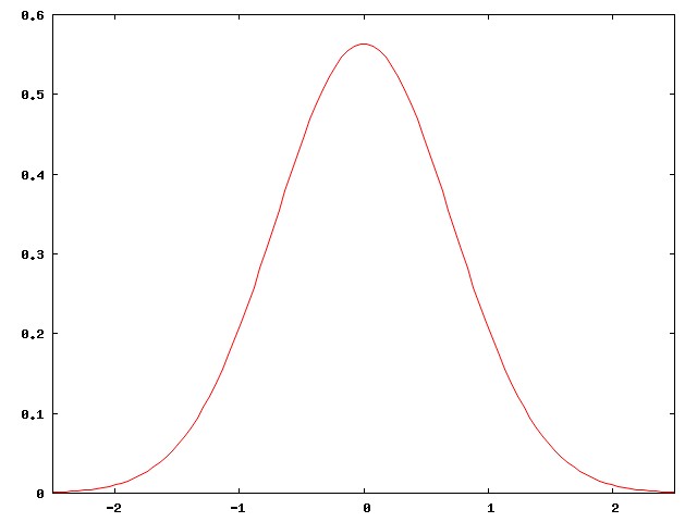
But major-league baseball players are not the general population. They are carefully selected, among the best of the best. They are all chosen from the right-hand edge of the normal curve. The people in the middle of the normal curve, people like me, play baseball in Clark Park, not in Quankee Stadium.
Here's the right-hand corner of the curve above, highly magnified:
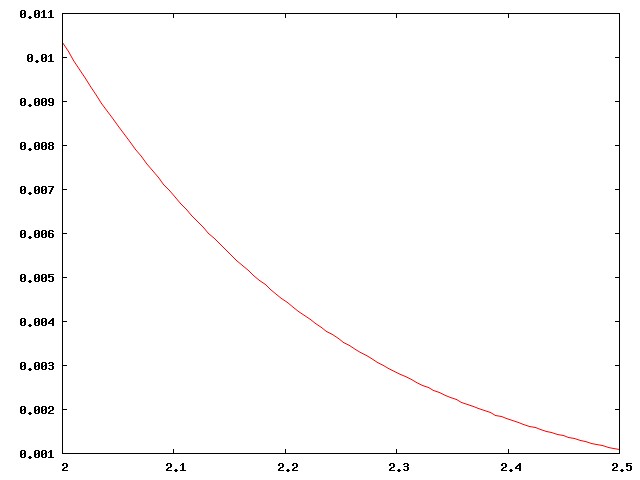
Actually I didn't present the case strongly enough. There are around 800 regular major-league ballplayers in the USA, drawn from a population of around 300 million, a ratio of one per 375,000. Well, no, the ratio is smaller, since the U.S. leagues also draw the best players from Mexico, Venezuela, Canada, the Dominican Republic, Japan, and elsewhere. The curve above is much too inclusive. The real curve for major-league ballplayers looks more like this:
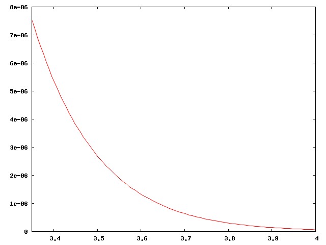
This has important implications for the analysis of baseball. A player who is "merely" above average is a rare and precious resource, to be cherished; far more players are below average. Skilled analysts know that comparisons with the "average" player are misleading, because baseball is full of useful, effective players who are below average. Instead, analysts compare players to a hypothetical "replacement level", which is effectively the leftmost edge of the curve, the level at which a player can be easily replaced by one of those kids from triple-A ball.
In the Historical Baseball Abstract, Bill James describes some great team, I think one of the Cincinnati Big Red Machine teams of the mid-1970s, as "possibly the only team in history that was above average at every position". That's an important thing to know about the sport, and about team sports in general: you don't need great players to completely clobber the opposition; it suffices to have players that are merely above average. But if you're the coach, you'd better learn to make do with a bunch of players who are below average, because that's what you have, and that's what the other team will beat you with.
The right-skewedness of the right side of a normal distribution has implications that are important outside of baseball. Stephen Jay Gould wrote an essay about how he was diagnosed with cancer and given six months to live. This sounds awful, and it is awful. But six months was the expected lifetime for patients with his type of cancer—the average remaining lifetime, in other words—and in fact, nearly everyone with that sort of cancer lived less than six months, usually much less. The average was only skewed up as high as six months because of a few people who took years to die. Gould realized this, and then set about trying to find out how the few long-lived outliers survived and what he could do to turn himself into one of the long-lived freaks. And he succeeded, and lived for twenty years, dying eventually at age 60.
My heavens, I just realized that what I've written is an article about the "long tail". I had no idea I was being so trendy. Sorry, everyone.
[Other articles in category /math] permanent link